22.4 - Tangents And Normals

In the previous section, we completed a discussion on the Derivative test which help us to find whether a given function is increasing or decreasing. In this section, we will see Tangents and Normals.

Some basic details can be written in 9 steps:
1. In analytic geometry classes, we saw that:
Equation of a straight line passing through (x₀,y₀) is given by
y – y₀ = m(x – x₀)
    ♦ Here m is the slope of that straight line.
2. So if we know the slope m, we can easily write the equation of the straight line passing through any given point (x₀,y₀).
3. Now consider a curve given by y = f(x).
• We have seen numerous curves of this type, in the previous sections.
• For example, f(x) = x³ – 3x² + 3 is a curve.
• If we want to plot that curve on the xy-plane, we can write:
y = x³ – 3x² + 3
4. Mark some random points on any given curve. Draw tangents through each of those points. We know that, no two tangents will be the same. This is because each tangent will have it’s own slope.
5. Suppose that, we want a tangent at a particular point (x₀,y₀).
• Based on (1) and (2) above, we can easily draw that tangent if we know the slope of the tangent at (x₀,y₀)
• But the slope of the tangent at (x₀,y₀) is f'(x₀).
• So the equation of the required tangent is:
y – y₀ = f'(x₀)(x – x₀)
6. Now we can write the equation of the normal also at (x₀,y₀).
• For that, we make use of the following fact:
Slope of the perpendicular line is the negative reciprocal of the slope of the original line.
• We can write:
Equation of the required normal is:
$\rm{y - y_0 \,=\,\frac{-1}{f'(x_0)} (x - x_0)}$
7. Suppose that, f'(x₀) = 0
• Then it means that, the tangent at (x₀,y₀) is parallel to the x-axis.
• In such a situation, we can straight away write the equation of the tangent at (x₀,y₀) as: y = y₀
8. Suppose that, f'(x₀) tends to ∞.
• Then it means that, the tangent at (x₀,y₀) tends to be parallel to the y-axis.
• In such a situation, we can straight away write the equation of the tangent at (x₀,y₀) as: x = x₀
9. The following information will be very useful while solving some types of problems. It can be written in 2 steps:
(i) If 𝜃 is the angle which a straight line makes with the +ve direction of the x-axis, then slope of that straight line will be equal to tan 𝜃. (We saw this in analytic geometry classes)
(ii) So we can write:
If the tangent at (x₀,y₀) makes an angle 𝜃 with the +ve direction of the x-axis, then f'(x₀) = tan 𝜃.

---

Now we will see some solved examples:
Solved example 22.14
Find the slope of the tangent to the curve y = x³ − x at x = 2
Solution:
• Slope of the tangent at x = 2 is $\rm{\left. \frac{dy}{dx} \right |_{x = 2}}$
• It can be calculated as shown below:

• The graphs are shown in fig.22.14 below.
    ♦ The curve is drawn in red color.
    ♦ The tangent at x = 2 is drawn in green color.

Fig.22.14

• We see that, slope of the green line is 11.

Solved example 22.15
Find the point at which the tangent to the curve $\rm{y = \sqrt{4x – 3} ~-~1}$ has its slope $\rm{\frac{2}{3}}$.
Solution:
1. The derivative can be used to find the slope of tangent at any point. So we will first find the derivative.

2. The slope must be 2/3. So we can write:

3. Equation of the curve is: $\rm{y = \sqrt{4x – 3} ~-~1}$
• When x = 3, we get:
$\rm{y = \sqrt{4(3) – 3} ~-~1}~=~2$

4. Therefore, we can write:
Mark the point (3,2) on the given curve. Draw the tangent at that point. Slope of that tangent will be 2/3.

• The graph is shown in fig.22.15 below:
    ♦ The curve is drawn in red color.
    ♦ The tangent at (3,2) is drawn in green color.

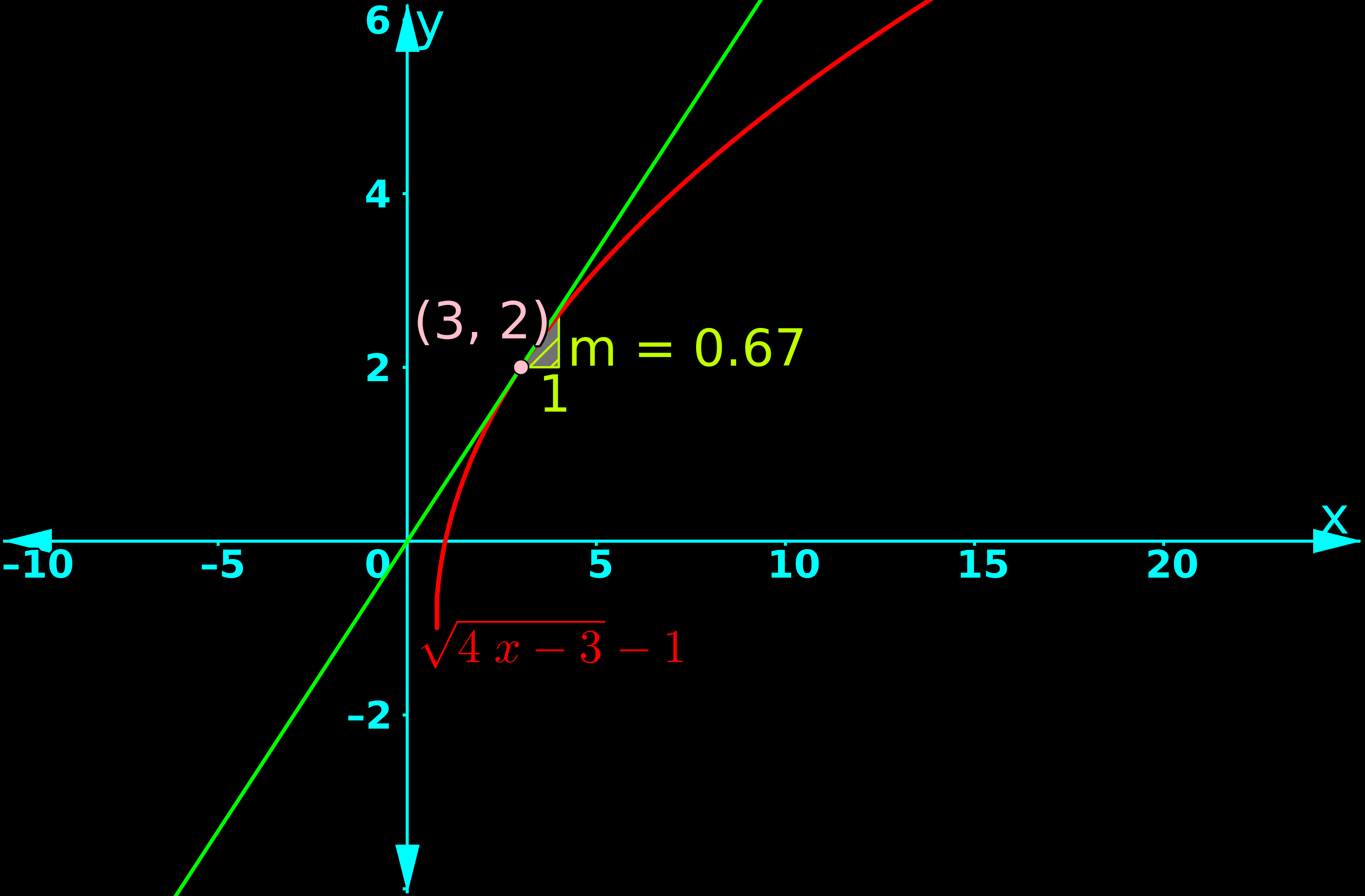
Fig.22.15

• We see that, slope of the green line is 2/3 = 0.67

Note: In the above graph, we do not see much red curve below the x-axis. The reason can be written in 4 steps:
(i) When x = 3, we can write:
$\rm{y = \sqrt{4(3) – 3} ~-~1}~=~(\pm 3 -1)~=~2~\text{OR}~-4$
So (3, −4) is a possible point on the graph. But it is not plotted.
(ii) Another example:
When x = 7, we can write:
$\rm{y = \sqrt{4(7) – 3} ~-~1}~=~(\pm 5 -1)~=~4~\text{OR}~-6$
So (7, −6) is a possible point on the graph. But it is not plotted.
(iii) We do not plot such points. If we do, then it means that, for inputs like x = 3, 7 etc., there will be two outputs.
• If there are two outputs, we cannot call it a function.
(iv) So we restrict the output values (range).

Solved example 22.16
Find the equation of all lines having slope 2 and being tangent to the curve $\rm{y + \frac{2}{x - 3}~=~0}$.
Solution:
1. The derivative can be used to find the slope of tangent at any point. So we will first find the derivative.

2. The slope must be 2. So we can write:

3. Equation of the curve is: $\rm{y + \frac{2}{x - 3}~=~0}$
• When x = 4, we get:
$\rm{y = \frac{2}{3 - x}~=~\frac{2}{3 - 4}~=~-2}$
• When x = 2, we get:
$\rm{y = \frac{2}{3 - x}~=~\frac{2}{3 - 2}~=~2}$

4. Therefore, we can write:
There are two points (4,−2) and (2,2). Mark those two points on the given curve. Draw the tangent at each of those points. The two tangents will be parallel to each other with a slope of 2.

• The graph is shown in fig.22.16 below:
    ♦ The curve is drawn in red color.
    ♦ The tangents are drawn in green color.

Fig.22.16

• We see that, slope of the green lines is 2

5. Now we want the equation of the two tangents. We can use the general equation:
y – y₀ = m(x – x₀)
• So the equation of the tangent through (2,2) is:
y – 2 = 2(x – 2)
⇒ y − 2 = 2x − 4
⇒ y − 2x + 2 = 0
• Similarly, the equation of the tangent through (4,−2) is:
y – (−2) = 2(x – 4)
⇒ y + 2 = 2x − 8
⇒ y − 2x + 10 = 0

Solved example 22.17
Find points on the curve $\rm{\frac{x^2}{4}\,+\,\frac{y^2}{25}\,=\,1}$ at which tangents are (i) parallel to x-axis (ii) parallel to y-axis.
Solution:
• The derivative can be used to find the slope of tangent at any point. So we will first find the derivative.

Part (i): Tangents parallel to x-axis
1. Consider the points where tangents are parallel to the x-axis.
• Those tangents will have a slope of zero. So we can write:

2. When x = 0, we get:

3. So the points are: (0,5) and (0,−5)
The tangents at these points are parallel to the x-axis.

• The graph is shown in fig.22.16 below:
    ♦ The curve is drawn in red color.
    ♦ The tangents are drawn in green color.

Fig.22.17

Part (ii): Tangents parallel to y-axis
1. Consider the points where tangents are parallel to the y-axis.
• The normals at those points will have a slope of zero. Slope of normal is the negative reciprocal of that of tangent. So we can write:

2. When y = 0, we get:

3. So the points are: (2,0) and (−2,0)
• The normals at these points are parallel to the x-axis.
• Consequently, the tangents at these points are parallel to the y-axis. They are drawn in magenta color in fig.22.17 above.

---

In the next section, we will see a few more solved examples.

Previous

Contents

Next

Copyright©2024 Higher secondary mathematics.blogspot.com

Chapter 13.13 - Derivative as a Function

In the previous section, we saw an easy method to find the derivative at a point. In this section, we will see a general form.

• The general form can be obtained using the same fig.13.30 that we saw in the previous section. All we need to do is, change 'a' to 'x'.
• The steps are the same with 'x' in place of 'a'. However, we will write all those 11 steps here:
1. In fig.13.31 below, the red curve is the graph of f(x).

Fig.13.31

• Two points P and Q are marked on the red curve.
(P is an arbitrary point. An arbitrary point is chosen so that, it will be applicable for all cases. The dictionary meaning of the word "arbitrary" can be seen here) 
    ♦ A green horizontal line is drawn through P.
    ♦ A green vertical line is drawn through Q.
    ♦ These horizontal and vertical lines meet at R
• Thus we get a right triangle PQR
2. A green dashed vertical line is drawn through P.
• This vertical line meets the x-axis at (x,0)
[We are able to write "(x,0)" because, P is an arbitrary point. Since it is an arbitrary point, 'x' can be any point in the domain of f(x)]
• So we can write:
The x-coordinate of P is ‘x’.
• If the x-coordinate is ‘x’, then obviously, the y-coordinate will be f(x)
• Thus we get the coordinates of P: (x,f(x))
3. Another green dashed vertical line is drawn through R.
• This vertical line meets the x-axis at ((x+h),0)
• So we can write:
The x-coordinate of Q is ‘(x+h)’.
• If the x-coordinate is ‘(x+h)’, then obviously, the y-coordinate will be f(x+h)
• Thus we get the coordinates of Q: ((x+h),f(x+h))
4. Using the x-coordinates of P and Q, we can find the horizontal distance between P and Q.
• We get:
Horizontal distance between P and Q = [(x+h) – x] = h
• That means, the length PR = h.
5.  Using the y-coordinates of P and Q, we can find the vertical distance between P and Q.
• We get:
Vertical distance between P and Q = [f(x+h) – f(x)]
• That means, the length QR = [f(x+h) – f(x)].
6. Now we have the base and altitude of the right triangle PQR.
• So we can write the slope of the line PQ.
Slope of PQ = $\frac{[f(x+h) – f(x)]}{h}$
7. If Q is brought very close to P, then the slope calculated in (6) will be the slope of the tangent at P
• For bringing Q closer to P, we must decrease the length h. When h approaches zero, Q will be very close to P.
• h must become very close to zero. At the same time, it must not become exact zero. This can be written as:
$\lim_{h\rightarrow 0} h$
8. From (5), we have the length of the altitude:
[f(x+h) – f(x)]
• When h approaches zero, the base PR will become infinitesimal.
• There will be corresponding changes in the altitude also.
• When h approaches zero, the length of the altitude can be written as: $\lim_{h\rightarrow 0} {[f(x+h) – f(x)]}$
9. So now we can write the slope of the tangent at P:
$\frac{\lim_{h\rightarrow 0} {[f(x+h) – f(x)]}}{\lim_{h\rightarrow 0} h}$
• The limit is being applied to both numerator and denominator. So this can be written in a simplified form as:
Slope of tangent at P = $\lim_{h\rightarrow 0}{\left[\frac{f(x+h) – f(x)}{h} \right]}$
10. But slope of the tangent at P is the derivative at P.
• Point P corresponds to any x in the domain.
• So we can write:
The result in (9) gives the derivative of f(x) at any x in the domain.
11. The derivative of f(x) at x is denoted as: f'(x).
• So we can write:
$$f'(x)~=~\lim_{h\rightarrow 0}{\left[\frac{f(x+h) – f(x)}{h} \right]}$$

---

Now we will see the same solved examples of the previous section:
Solved example 13.6
Find the derivative of f(x) = 3x.
Solution:
• In our present case, f(x) = 3x. So we get:
$\begin{array}{ll}
{}&{f'(x)}
& {~=~}& {\lim_{h\rightarrow 0}{\left[\frac{f(x+h) – f(x)}{h} \right]}}
&{} \\

{}&{}
& {~=~}& {\lim_{h\rightarrow 0}{\left[\frac{3(x+h) – 3 x}{h} \right]}}
&{} \\

{}&{}
& {~=~}& {\lim_{h\rightarrow 0}{\left[\frac{3x + 3h – 3x}{h} \right]}}
&{} \\

{}&{}
& {~=~}& {\lim_{h\rightarrow 0}{\left[\frac{3h}{h} \right]}}
&{} \\

{}&{}
& {~=~}& {3 \lim_{h\rightarrow 0}{\left[\frac{h}{h} \right]}}
&{} \\

{}&{}
& {~=~}& {3 \lim_{h\rightarrow 0}{1}}
&{} \\

{}&{}
& {~=~}& {3 × 1}
&{} \\

{}&{}
& {~=~}& {3}
&{} \\

\end{array}$

Solved example 13.7
Find the derivative of f(x) = 2x² + 3x - 5. Also prove that f'(0) + 3f'(-1) = 0
Solution:
Part (i):
• In our present case, f(x) = 2x² + 3x - 5. So we get:
$\begin{array}{ll}
{}&{f'(x)}
& {~=~}& {\lim_{h\rightarrow 0}{\left[\frac{f(x+h) – f(x)}{h} \right]}}
&{} \\

{}&{}
& {~=~}& {\lim_{h\rightarrow 0}{\left[\frac{[2(x+h)^2 + 3(x+h) - 5] – [2×(x)^2 + 3 x ~- 5]}{h} \right]}}
&{} \\

{}&{}
& {~=~}& {\lim_{h\rightarrow 0}{\left[\frac{[2(x^2 + 2hx + h^2) + 3x +3h - 5] – [2 x^2 + 3x - 5]}{h} \right]}}
&{} \\

{}&{}
& {~=~}& {\lim_{h\rightarrow 0}{\left[\frac{2x^2 + 4hx + 2h^2 + 3x + 3h - 5 – 2 x^2 - 3x + 5}{h} \right]}}
&{} \\

{}&{}
& {~=~}& {\lim_{h\rightarrow 0}{\left[\frac{4hx + 2h^2 + 3h}{h} \right]}}
&{} \\

{}&{}
& {~=~}& {\lim_{h\rightarrow 0}{\left[\frac{h(2h +4x + 3)}{h} \right]}}
&{} \\

{}&{}
& {~=~}& {\lim_{h\rightarrow 0}{[2h + 4x +3]}}
&{} \\

{}&{}
& {~=~}& {4x + 3}
&{} \\

\end{array}$

Part (ii):
1. We have: f'(x) = 4x + 3
2. Thus we get: f'(0) = [4(0) + 3] = 3
3. Also we get: f'(-1) = [4(-1) + 3] = [-4 + 3] = -1
4. So f'(0) + 3f'(-1) = [3 + 3(-1)] = [3 - 3] = 0

◼ A graphical description can be written in 3 steps:
1. In the fig.13.32 below, f(x) = 2x² + 3x - 5 is plotted in red color.

Fig.13.32

2. We saw that: f'(0) = 3
• That means, the "derivative of f(x)" at (x = 0) is 3.
    ♦ That means, slope of the tangent at (x = 0) is 3.
• When (x=0), f(x) is -5.
    ♦ So we mark the point (0,-5)
• If we have a point and the slope, we can draw a line through that point (recall the slope-point form that we saw in coordinate geometry lessons).
• So we draw a line through (0,-5) at a slope of 3.
    ♦ This line will be the tangent of f(x) at (x=0).
    ♦ This tangent is shown in green color.
3. We saw that: f'(-1) = -1
• That means, the "derivative of f(x)" at (x = -1) is -1.
    ♦ That means, slope of the tangent at (x = -1) is -1.
• When (x=-1), f(x) is -6.
    ♦ So we mark the point (-1,-6)
• If we have a point and the slope, we can draw a line through that point (recall the slope-point form that we saw in coordinate geometry lessons).
• So we draw a line through (-1,-5) at a slope of -1.
    ♦ This line will be the tangent of f(x) at (x=-1).
    ♦ This tangent is shown in white color.

Solved example 13.8
Find the derivative of sin x
Solution:
• In our present case, f(x) = sin x. So we get:
$\begin{array}{ll}
{}&{f'(x)}
& {~=~}& {\lim_{h\rightarrow 0}{\left[\frac{f(x+h) – f(x)}{h} \right]}}
&{} \\

{}&{}
& {~=~}& {\lim_{h\rightarrow 0}{\left[\frac{[\sin (x+h)] – [sin x]}{h} \right]}}
&{} \\

{}&{}
& {~=~}& {\lim_{h\rightarrow 0}{\left[\frac{[\sin x \cos h ~+~\cos x \sin h] – [sin x]}{h} \right]}}
&{} \\

{}&{}
& {~=~}& {\lim_{h\rightarrow 0}{\left[\frac{\sin x (\cos h - 1)~+~ \cos x \sin h}{h} \right]}}
&{} \\

{}&{}
& {~=~}& {\lim_{h\rightarrow 0}{\left[\frac{\sin x (\cos h - 1)}{h} \right]}~+~\lim_{h\rightarrow 0}{\left[\frac{\cos x \sin h}{h} \right]}}
&{} \\

{}&{}
& {~=~}& {\sin x \lim_{h\rightarrow 0}{\left[\frac{\cos h - 1}{h} \right]}~+~\cos x \lim_{h\rightarrow 0}{\left[\frac{\sin h}{h} \right]}}
&{} \\

{}&{}
& {~=~}& {\sin x × 0~+~\cos x × 1}
&{} \\

{}&{}
& {~=~}& {\cos x}
&{} \\

\end{array}$

◼ Let us find the derivatives at some convenient points:
• We have: f'(x) = cos x
• Let us find the derivative at (x = 0) and $\rm{\left(x = \frac{\pi}{3} \right)}$. We get:
    ♦ f'(0) = cos 0 = 1
    ♦ $\rm{f' \left(\frac{\pi}{3}\right)~=~\cos \left(\frac{\pi}{3}\right)~=~\frac{1}{2}}$

◼ A graphical description can be written in 3 steps:
1. In the fig.13.33 below, f(x) = sin x is plotted in red color.

Fig.13.33

2. We saw that: f'(0) = 1
• That means, the "derivative of f(x)" at (x = 0) is 1.
    ♦ That means, slope of the tangent at (x = 0) is 1.
• When (x=0), f(x) is sin 0 = 0.
    ♦ So we mark the point (0,0)
• If we have a point and the slope, we can draw a line through that point (recall the slope-point form that we saw in coordinate geometry lessons).
• So we draw a line through (0,0) at a slope of 1.
    ♦ This line will be the tangent of f(x) at (x=0).
    ♦ This tangent is shown in green color.
3. We saw that: $\rm{f' \left(\frac{\pi}{3}\right)~=~\frac{1}{2}}$
• That means, the "derivative of f(x)" at $\rm{\left(x = \frac{\pi}{3} \right)}$ is $\frac{1}{2}$
    ♦ That means, slope of the tangent at $\rm{\left(x = \frac{\pi}{3} \right)}$ is $\frac{1}{2}$.
• When $\rm{\left(x = \frac{\pi}{3} \right)}$, f(x) is $\frac{\sqrt3}{2}$.
    ♦ So we mark the point $\rm{\left(\frac{\pi}{3}, \frac{\sqrt3}{2} \right)}$
• If we have a point and the slope, we can draw a line through that point (recall the slope-point form that we saw in coordinate geometry lessons).
• So we draw a line through $\rm{\left(\frac{\pi}{3}, \frac{\sqrt3}{2} \right)}$ at a slope of $\frac{1}{2}$.
    ♦ This line will be the tangent of f(x) at $\rm{\left(x = \frac{\pi}{3} \right)}$.
    ♦ This tangent is shown in white color.

Solved example 13.9
Find the derivative of f(x) = 3. Also find f'(0) and f'(3). 
Solution:
Part (i):
• In our present case, f(x) = 3. So we get:

$\begin{array}{ll}
{}&{f'(0)}
& {~=~}& {\lim_{h\rightarrow 0}{\left[\frac{f(x+h) – f(x)}{h} \right]}}
&{} \\

{}&{}
& {~=~}& {\lim_{h\rightarrow 0}{\left[\frac{[3] – [3]}{h} \right]}}
&{} \\

{}&{}
& {~=~}& {\lim_{h\rightarrow 0}{\left[\frac{0}{h} \right]}}
&{} \\

{}&{}
& {~=~}& {0}
&{} \\

\end{array}$

Part (ii):
1. We have: f'(x) = 0. This is a constant function.
• So f'(0) = 0.
2. We have: f'(x) = 0. This is a constant function.
• So f'(3) = 0.

◼ In this example, we see that:
    ♦ f’(0) = 0
    ♦ f’(3) = 0
• In fact, we can put any value for a. The derivative will be zero.
• The reason can be written in 2 steps:
1. f(x) = 3 is a constant function.
• That means, whatever be the value of x, the resulting f(x) will be the same.
• If there is no change in f(x), it means that, there is no rate of change.
    ♦ That means, rate of change is zero.
    ♦ That means, derivative is zero.
2. We can think in terms of slope of tangent also.
• For a straight line, the tangent at any point, will be the line itself.
• Here, the straight line is horizontal. So the tangent at any point will also be horizontal.
• For a horizontal line, the slope is zero.

---

• For a given function f, we can find the derivative at every point. The derivative will be a new function denoted by f'.
• In some cases, the derivative will be a constant function.
    ♦ The derivative in solved example 13.6 above is a constant function.
    ♦ The derivative in solved example 13.9 above is a constant function.
• In some cases, the derivative will be an ordinary function.
    ♦ The derivative in solved example 13.7 above is an ordinary function.
    ♦ The derivative in solved example 13.8 above is an ordinary function.

---

◼ Derivative can be denoted in different ways. In the discussions above, we denoted it as f'(x)
• Five more methods are given below:
1. Derivative can be denoted as $\frac{d}{dx}\left(f(x) \right)$.
2. If y = f(x), then the derivative can be denoted as $\frac{dy}{dx}$.
• We can read it in any one of the two ways below:
(i) Derivative of y with respect to x.
(ii) "dy" by "dx"
3. Derivative can be denoted as : $D \left(f(x) \right)$.
4. Derivative of f(x) at (x=a) can be denoted in any one of the three ways below:
(i) $\left.\frac{d}{dx} f(x)\right\vert_{a}$

(ii) $\left.\frac{df}{dx}\right\vert_{a}$

(iii) $\left(\frac{df}{dx}\right)_{x=a}$

---

In the next section, we will see a few more solved examples.

Previous

Contents

Next

Copyright©2023 Higher secondary mathematics.blogspot.com

Chapter 13.12 - Method to Find Derivative

In the previous section, we saw that derivative at a point, is the slope of the tangent at that point. In the section before that, we saw derivative as the rate of change. In this section, we will see an easy method to find the derivative at any given point.

It can be written in 11 steps:
1. In fig.13.30 below, the red curve is the graph of f(x).

Fig.13.30

• Two points P and Q are marked on the red curve.
    ♦ A green horizontal line is drawn through P.
    ♦ A green vertical line is drawn through Q.
    ♦ These horizontal and vertical lines meet at R
• Thus we get a right triangle PQR
2. A green dashed vertical line is drawn through P.
• This vertical line meets the x-axis at (a,0)
• So we can write:
The x-coordinate of P is ‘a’.
• If the x-coordinate is ‘a’, then obviously, the y-coordinate will be f(a)
• Thus we get the coordinates of P: (a,f(a))
3. Another green dashed vertical line is drawn through R.
• This vertical line meets the x-axis at ((a+h),0)
• So we can write:
The x-coordinate of Q is ‘(a+h)’.
• If the x-coordinate is ‘(a+h)’, then obviously, the y-coordinate will be f(a+h)
• Thus we get the coordinates of Q: ((a+h),f(a+h))
4. Using the x-coordinates of P and Q, we can find the horizontal distance between P and Q.
• We get:
Horizontal distance between P and Q = [(a+h) – a] = h
• That means, the length PR = h.
5.  Using the y-coordinates of P and Q, we can find the vertical distance between P and Q.
• We get:
Vertical distance between P and Q = [f(a+h) – f(a)]
• That means, the length QR = [f(a+h) – f(a)].
6. Now we have the base and altitude of the right triangle PQR.
• So we can write the slope of the line PQ.
Slope of PQ = $\frac{[f(a+h) – f(a)]}{h}$
7. If Q is brought very close to P, then the slope calculated in (6) will be the slope of the tangent at P
• For bringing Q closer to P, we must decrease the length h. When h approaches zero, Q will be very close to P.
• h must become very close to zero. At the same time, it must not become exact zero. This can be written as:
$\lim_{h\rightarrow 0} h$
8. From (5), we have the length of the altitude:
[f(a+h) – f(a)]
• When h approaches zero, the base PR will become infinitesimal.
• There will be corresponding changes in the altitude also.
• When h approaches zero, the length of the altitude can be written as: $\lim_{h\rightarrow 0} {[f(a+h) – f(a)]}$
9. So now we can write the slope of the tangent at P:
$\frac{\lim_{h\rightarrow 0} {[f(a+h) – f(a)]}}{\lim_{h\rightarrow 0} h}$
• The limit is being applied to both numerator and denominator. So this can be written in a simplified form as:
Slope of tangent at P = $\lim_{h\rightarrow 0}{\left[\frac{f(a+h) – f(a)}{h} \right]}$
10. But slope of the tangent at P is the derivative at P.
• Point P corresponds to (x = a)
• So we can write:
The result in (9) gives the derivative of f(x) at (x = a).
11. The derivative of f(x) at (x=a) is denoted as: f'(a).
• So we can write:
$$f'(a)~=~\lim_{h\rightarrow 0}{\left[\frac{f(a+h) – f(a)}{h} \right]}$$

---

Now we will see some solved examples:
Solved example 13.6
Find the derivative at x = 2 of the function f(x) = 3x.
Solution:
1. We have: $f'(a)~=~\lim_{h\rightarrow 0}{\left[\frac{f(a+h) – f(a)}{h} \right]}$
2. In our present case, a = 2 and f(x) = 3x.
• So we get:
$\begin{array}{ll}
{}&{f'(2)}
& {~=~}& {\lim_{h\rightarrow 0}{\left[\frac{f(2+h) – f(2)}{h} \right]}}
&{} \\

{}&{}
& {~=~}& {\lim_{h\rightarrow 0}{\left[\frac{3(2+h) – 3 × 2}{h} \right]}}
&{} \\

{}&{}
& {~=~}& {\lim_{h\rightarrow 0}{\left[\frac{6 + 3h – 6}{h} \right]}}
&{} \\

{}&{}
& {~=~}& {\lim_{h\rightarrow 0}{\left[\frac{3h}{h} \right]}}
&{} \\

{}&{}
& {~=~}& {3 \lim_{h\rightarrow 0}{\left[\frac{h}{h} \right]}}
&{} \\

{}&{}
& {~=~}& {3 \lim_{h\rightarrow 0}{1}}
&{} \\

{}&{}
& {~=~}& {3 × 1}
&{} \\

{}&{}
& {~=~}& {3}
&{} \\

\end{array}$

3. We see that the derivative is '3'.
• So we can write:
At the point where (x = 2), the rate of change of y with respect to x is 3.
• In fact, for this problem, the rate of change at every point will be 3.
4. We see that the derivative is '3'.
• So we can write:
At the point where (x = 2), the slope of the tangent is 3.
• In fact, for this problem, the slope of tangent at any point will be 3. The reason can be written in steps:
(i) For a straight line, the tangent at any point, will be the line itself.
(ii) Here, the slope of the line is 3. So the tangent at any point will also have the slope 3

Solved example 13.7
Find the derivative of the function f(x) = 2x² + 3x - 5 at x = -1. Also prove that f'(0) + 3f'(-1) = 0
Solution:
Part (i):
1. We have: $f'(a)~=~\lim_{h\rightarrow 0}{\left[\frac{f(a+h) – f(a)}{h} \right]}$
2. In our present case, a = -1 and f(x) = 2x² + 3x - 5 .
• So we get:
$\begin{array}{ll}
{}&{f'(-1)}
& {~=~}& {\lim_{h\rightarrow 0}{\left[\frac{f(-1+h) – f(-1)}{h} \right]}}
&{} \\

{}&{}
& {~=~}& {\lim_{h\rightarrow 0}{\left[\frac{[2(-1+h)^2 + 3(-1+h) - 5] – [2×(-1)^2 + 3 × -1 - 5]}{h} \right]}}
&{} \\

{}&{}
& {~=~}& {\lim_{h\rightarrow 0}{\left[\frac{[2(1 - 2h + h^2) + (-3+3h) - 5] – [2 - 3 - 5]}{h} \right]}}
&{} \\

{}&{}
& {~=~}& {\lim_{h\rightarrow 0}{\left[\frac{2 - 4h + 2h^2 -3+3h - 5 – 2 + 3 + 5}{h} \right]}}
&{} \\

{}&{}
& {~=~}& {\lim_{h\rightarrow 0}{\left[\frac{- h + 2h^2}{h} \right]}}
&{} \\

{}&{}
& {~=~}& {\lim_{h\rightarrow 0}{\left[\frac{h(2h - 1)}{h} \right]}}
&{} \\

{}&{}
& {~=~}& {\lim_{h\rightarrow 0}{[2h-1]}}
&{} \\

{}&{}
& {~=~}& {2 × 0~-~1}
&{} \\

{}&{}
& {~=~}& {-1}
&{} \\

\end{array}$

Part (ii):
1. We have: $f'(a)~=~\lim_{h\rightarrow 0}{\left[\frac{f(a+h) – f(a)}{h} \right]}$
2. In our present case, a = 0 and f(x) = 2x² + 3x - 5.
• So we get:
$\begin{array}{ll}
{}&{f'(0)}
& {~=~}& {\lim_{h\rightarrow 0}{\left[\frac{f(0+h) – f(0)}{h} \right]}}
&{} \\

{}&{}
& {~=~}& {\lim_{h\rightarrow 0}{\left[\frac{[2(0+h)^2 + 3(0+h) - 5] – [2×(0)^2 + 3 × 0 ~- 5]}{h} \right]}}
&{} \\

{}&{}
& {~=~}& {\lim_{h\rightarrow 0}{\left[\frac{[2h^2 + 3h) - 5] – [2×0 + 3 × 0 ~- 5]}{h} \right]}}
&{} \\

{}&{}
& {~=~}& {\lim_{h\rightarrow 0}{\left[\frac{2h^2 + 3h - 5 + 5}{h} \right]}}
&{} \\

{}&{}
& {~=~}& {\lim_{h\rightarrow 0}{\left[\frac{2h^2 + 3h}{h} \right]}}
&{} \\

{}&{}
& {~=~}& {\lim_{h\rightarrow 0}{\left[\frac{h(2h + 3)}{h} \right]}}
&{} \\

{}&{}
& {~=~}& {\lim_{h\rightarrow 0}{\left[2h + 3 \right]}}
&{} \\

{}&{}
& {~=~}& {2 × 0 ~+ 3}
&{} \\

{}&{}
& {~=~}& {3}
&{} \\

\end{array}$

Part (iii):
1. From part (i), we have: f'(-1) = -1
2. From part (ii), we have: f'(0) = 3
3. So we get:
f'(0) + 3f'(-1) = [3 + (3 × -1)] = [3 - 3] = 0

---

At this stage, we are able to understand an important fact. It can be written in 2 steps:
(i) In the previous sections, we saw that:
Limits are subjected to various rules.
(ii) Those rules can be effectively used to evaluate the derivative.

---

Solved example 13.8
Find the derivative of sin x at x = 0
Solution:
1. We have: $f'(a)~=~\lim_{h\rightarrow 0}{\left[\frac{f(a+h) – f(a)}{h} \right]}$
2. In our present case, a = 0 and f(x) = sin x.
• So we get:
$\begin{array}{ll}
{}&{f'(0)}
& {~=~}& {\lim_{h\rightarrow 0}{\left[\frac{f(0+h) – f(0)}{h} \right]}}
&{} \\

{}&{}
& {~=~}& {\lim_{h\rightarrow 0}{\left[\frac{[\sin (0+h)] – [sin 0]}{h} \right]}}
&{} \\

{}&{}
& {~=~}& {\lim_{h\rightarrow 0}{\left[\frac{[\sin h] – [sin 0]}{h} \right]}}
&{} \\

{}&{}
& {~=~}& {\lim_{h\rightarrow 0}{\left[\frac{[\sin h] – [0]}{h} \right]}}
&{} \\

{}&{}
& {~=~}& {\lim_{h\rightarrow 0}{\left[\frac{\sin h}{h} \right]}}
&{} \\

{}&{}
& {~=~}& {1}
&{} \\

\end{array}$

Solved example 13.9
Find the derivative of f(x) = 3 at x = 0 and at x = 3
Solution:
Part (i):
1. We have: $f'(a)~=~\lim_{h\rightarrow 0}{\left[\frac{f(a+h) – f(a)}{h} \right]}$
2. In our present case, a = 0 and f(x) = 3.
• So we get:
$\begin{array}{ll}
{}&{f'(0)}
& {~=~}& {\lim_{h\rightarrow 0}{\left[\frac{f(0+h) – f(0)}{h} \right]}}
&{} \\

{}&{}
& {~=~}& {\lim_{h\rightarrow 0}{\left[\frac{[3] – [3]}{h} \right]}}
&{} \\

{}&{}
& {~=~}& {\lim_{h\rightarrow 0}{\left[\frac{0}{h} \right]}}
&{} \\

{}&{}
& {~=~}& {0}
&{} \\

\end{array}$

Part (ii):
1. We have: $f'(a)~=~\lim_{h\rightarrow 0}{\left[\frac{f(a+h) – f(a)}{h} \right]}$
2. In our present case, a = 3 and f(x) = 3.
• So we get:
$\begin{array}{ll}
{}&{f'(3)}
& {~=~}& {\lim_{h\rightarrow 0}{\left[\frac{f(3+h) – f(3)}{h} \right]}}
&{} \\

{}&{}
& {~=~}& {\lim_{h\rightarrow 0}{\left[\frac{[3] – [3]}{h} \right]}}
&{} \\

{}&{}
& {~=~}& {\lim_{h\rightarrow 0}{\left[\frac{0}{h} \right]}}
&{} \\

{}&{}
& {~=~}& {0}
&{} \\

\end{array}$

◼ In this example, we see that:
    ♦ f’(0) = 0
    ♦ f’(3) = 0
• In fact, we can put any value for a. The derivative will be zero.
• The reason can be written in 2 steps:
1. f(x) = 3 is a constant function.
• That means, whatever be the value of x, the resulting f(x) will be the same.
• If there is no change in f(x), it means that, there is no rate of change.
    ♦ That means, rate of change is zero.
    ♦ That means, derivative is zero.
2. We can think in terms of slope of tangent also.
• For a straight line, the tangent at any point, will be the line itself.
• Here, the straight line is horizontal. So the tangent at any point will also be horizontal.
• For a horizontal line, the slope is zero.

---

• Now we know how to find the derivative at any given point.
• It would be convenient if we could obtain a general form.
• For example, we saw that:
Derivative of 2x² + 3x -5 at (x = -1) is -1
• If we are asked to find the derivative of this function at say (x = 2), we will have to repeat all the steps using ‘2’.
• If we have a general form, we will be able to quickly find the derivative at any given point.
In the next section, we will see such a general form.

Previous

Contents

Next

Copyright©2023 Higher secondary mathematics.blogspot.com

Chapter 13.11 - Derivative as Slope of Tangent

In the previous section, we saw the basics about derivatives. We saw that, derivative is the rate of change. In this section, we will see another use of derivatives.

It can be written in 9 steps:
1. In fig.13.28 below, the red curve is the graph of a function f(x).

Fig.13.28

• C and D are two adjacent points on the graph.
• A yellow line connects C and D.
    ♦ A vertical green line is drawn through D.
    ♦ A horizontal green line is drawn through C.
• These vertical and horizontal green lines intersect at P.
• So we get a right triangle CPD
• We know that, slope of the line CD will be given by the ratio $\frac{\rm{PD}}{\rm{PC}}$
• The line CD intersects the red curve at two points  C and D
2. Keeping D fixed, let us consider a point which is closer to D
• This new point is marked as C₁ in the fig.13.28
    ♦ A horizontal green line is drawn through C₁
• Thus we get a right triangle C₁P₁D
• So slope of the line C₁D will be given by the ratio $\rm{\frac{P_1 D}{P_1 C_1}}$
• Note that:
    ♦ the denominator of this ratio
    ♦ is smaller than
    ♦ the denominator of the ratio in (1)
3. Keeping D fixed, let us consider a point which is still closer to D
• This new point is marked as C₂ in the fig.13.28
    ♦ A horizontal green line is drawn through C₂
• Thus we get a right triangle C₂P₂D
• So slope of the line C₂D will be given by the ratio $\rm{\frac{P_2 D}{P_2 C_2}}$
• Note that:
    ♦ the denominator of this ratio
    ♦ is smaller than
    ♦ the denominator of the ratio in (2)
4. Keeping D fixed, let us consider a point which is even more closer to D
• This new point is marked as C₃ in the fig.13.28
    ♦ A horizontal green line is drawn through C₃
• Thus we get a right triangle C₃P₃D
• So slope of the line C₃D will be given by the ratio $\rm{\frac{P_3 D}{P_3 C_3}}$
• Note that:
    ♦ the denominator of this ratio
    ♦ is smaller than
    ♦ the denominator of the ratio in (3)
5. Proceeding like this, we can mark points C₄, C₅, C₆, C₇ etc., which are closer and closer to D
• When the point is very close to D, the yellow line will no longer intersect the red curve at two points.
• The yellow line will intersect the red curve only at one point.
• When there is only one point, we can say that:
The yellow line touches the red curve.
• The ‘touch’ occurs at D
6. When the yellow line touches the red curve at D, we say that:
The yellow line is the tangent of the red curve at D
7. Even though there is only a "touch" at one point, we still have a triangle similar to CPD.
Only difference is that, the base of that triangle will be of infinitesimal length.
• Since there is a triangle, we can take the ratio $\rm{\frac{Altitude}{Base}}$. This ratio will give the slope.
• So we can write:
Slope of the tangent = $\frac{\text{PD corresponding to infinitesimal CP}}{\text{infinitesimal CP}}$.
(We use the word “corresponding: because:
For each length of the base CP, there will be a corresponding length for the altitude PD. Even when the base is infinitesimal, there will be a corresponding altitude)
8. But in the previous section, we saw that, the ratio with infinitesimal denominator is called the derivative.
• So we can write:
The slope of the tangent at a point is same as the derivative at that point.
9. We proved that, slope is equal to the derivative. We proved this by taking point C and moving forward towards D
• We can take point E and move backward towards D. We will get the same result. This is shown in fig.13.29 below:

Fig.13.29

• The reader should write all steps related to fig.13.29 and become convinced that slope is same as the derivative.

---

• We saw two applications of derivatives.
(i) Derivative as rate of change.
(ii) Derivative as slope of tangent.
• While discussing rate of change, we did not draw the line CD. Because, for that discussion, such a line is not required.
• But while discussing slope of tangent, we did draw that line. Because, it is that line CD which gradually becomes the tangent at D. This gradual change occurs when the point C becomes closer and closer to D.

---

In the next section, we will see an easy method to find the derivative. 

Previous

Contents

Next

Copyright©2023 Higher secondary mathematics.blogspot.com

Chapter 13.10 - Derivatives

In the previous section, we completed a discussion on limits. In this section, we will see a practical application of limits.

Some basics can be written in 23 steps:

1. Consider an object dropped from the top of a tall cliff.
• The distance (s) traveled by the object in time (t) is given by the formula:
s = 4.9t²
    ♦ distance should be measured in meters
    ♦ time should be measured in seconds.
2. Using this formula, we can get several ordered pairs in the form (t,s):
(i) When t = 0, the distance traveled is zero.
    ♦ Because, s = 4.9 × 0² = 0
    ♦ So we get the ordered pair (t,s) = (0,0)
(ii)  When t = 2, the distance traveled is 19.6 m.
    ♦ Because, s = 4.9 × 2² = 19.6 m
    ♦ So we get the ordered pair (t,s) = A(2,19.6)
(iii)  When t = 4, the distance traveled is 78.4 m.
    ♦ Because, s = 4.9 × 4² = 78.4 m
    ♦ So we get the ordered pair (t,s) = B(4,78.4)
(iv)  When t = 6, the distance traveled is 176.4 m.
    ♦ Because, s = 4.9 × 6² = 176.4 m
    ♦ So we get the ordered pair (t,s) = C(6,176.4)
(v)  When t = 8, the distance traveled is 313.6 m.
    ♦ Because, s = 4.9 × 2² = 313.6 m
    ♦ So we get the ordered pair (t,s) = D(8,313.6)
(vi)  When t = 10, the distance traveled is 490 m.
    ♦ Because, s = 4.9 × 10² = 490 m
    ♦ So we get the ordered pair (t,s) = E(10,490)
(vii)  When t = 12, the distance traveled is 705.6 m.
    ♦ Because, s = 4.9 × 12² = 705.6 m
    ♦ So we get the ordered pair (t,s) = F(12,705.6)
3. We can plot the above ordered pairs on a graph.
    ♦ t should be plotted along the x-axis.
    ♦ s should be plotted along the y-axis.
• Such a graph is shown in fig.13.25 below:

Fig.13.25

• The points representing the ordered pairs are connected using a smooth curve. In the above fig., the smooth curve is drawn in red color.
4. Now begins our task. The task can be explained in 3 steps:
(i) We know that, velocity of a freely falling body would be increasing continuously. It would be a uniformly increasing velocity.
(ii) The task is to find the velocity of the object when t = 8 s
(iii) That is., we want to know the velocity with which the object moves, at the instant when the reading in the stop-watch is 8 s.
5. For this task, we need to concentrate on the region near t = 8 s in the graph.
• That is., we need to concentrate on the region near point D.
• More specifically, we need to concentrate on the region between C and D.
• So we will enlarge the region between C and D. The enlarged portion is shown in fig.13.26 below:

Fig.13.26

6. Let us write two distances:
• From C we know that, when the stop-watch shows 6 s, the distance already fallen is 176.4 m.
• From D we know that, when the stop-watch shows 8 s, the distance already fallen is 313.6 m
7. So the distance fallen in the time duration of 2 s from C to D is (313.6 – 176.4) = 137.2 m
• We know that, average velocity multiplied by the " time duration of travel" will give the distance traveled.
• Let v_av(C-D) be the average velocity with which the object fell from C to D. Then we can write: 137.2 = v_av(C-D) × 2
• From this, we get: $v_{av(C-D)}~=~\frac{137.2}{2}$ = 68.6 m/s
8. Note that, average velocity is a ratio.
• Numerator of the ratio is: Distance fallen.
    ♦ It is the altitude PD of the right triangle CPD in fig.13.26
• Denominator of the ratio is: Time duration in which this distance is fallen.
    ♦ It is the base PC of the right triangle CPD in fig.13.26
◼ So we can write:
$v_{av(C-D)}~=~\frac{PD}{PC}~=~\frac{137.2}{2}$ = 68.6 m/s
9. We have the well known formula to find the velocity at any instant:
v = u + at
• Where:
    ♦ v is the velocity at time t
    ♦ u is the initial velocity
    ♦ a is the acceleration.
• In our present case,
    ♦ u is zero.
    ♦ a is the acceleration due to gravity, which is 9.8 m/s²
• So when time is 8 s, we get: v = 0 + 9.8 × 8 = 78.4 m/s
• This is very different from the average velocity obtained in (7) above.
10. So it seems that, the method of average velocity does not help us to obtain the velocity at D.
• But remember that, the time duration was taken as 2 s. The object would fall a large distance during this time. Consequently the velocity change will also be large.
• Let us try a smaller time duration.
11. Let us consider a new point C₁ between C and D. It corresponds to t = 7 s. This is shown in fig.13.27(a) below:

Fig.13.27

• When t = 7, the distance traveled is 240.1 m.
    ♦ Because, s = 4.9 × 7² = 240.1 m
    ♦ So we get the ordered pair (t,s) = A(7,240.1)
• So the duration from C₁ to D is (8-7) = 1 s
• The distance fallen from C₁ to D is (313.6 – 240.1) = 73.5 m
• Then the average velocity can be obtained as:
$v_{av(C_1 - D)}~=~\frac{P_1 D}{P_1 C_1}~=~\frac{73.5}{1}$ = 73.5 m/s
• This is closer to the actual value of 78.4 m/s that we obtained in (9)
12. Let us decrease the time duration further.
• Consider a new point C₂ between C₁ and D. It corresponds to t = 7.5 s
• When t = 7.5, the distance traveled is 240.1 m.
    ♦ Because, s = 4.9 × 7.5² = 275.6 m
    ♦ So we get the ordered pair (t,s) = A(7.5,275.6)
• So the duration from C₂ to D is (8-7.5) = 0.5 s
• The distance fallen from C₂ to D is (313.6 – 275.6) = 38.0 m
• Then the average velocity can be obtained as:
$v_{av(C_2 - D)}~=~\frac{P_2 D}{P_2 C_2}~=~\frac{38.0}{0.5}$ = 76.0 m/s
• This is even more closer to the actual value of 78.4 m/s that we obtained in (9)
13. Let us decrease the time duration further.
• Consider a new point C₃ between C₂ and D. It corresponds to t = 7.75 s
• When t = 7.75, the distance traveled is 240.1 m.
    ♦ Because, s = 4.9 × 7.5² = 294.3 m
    ♦ So we get the ordered pair (t,s) = A(7.75,294.3)
• So the duration from C₃ to D is (8-7.75) = 0.25 s
• The distance fallen from C₃ to D is (313.6 – 294.3) = 19.3 m
• Then the average velocity can be obtained as:
$v_{av(C_3 - D)}~=~\frac{P_3 D}{P_3 C_3}~=~\frac{19.3}{0.25}$ = 77.2 m/s
• This is even more closer to the actual value of 78.4 m/s that we obtained in (9)
14. Let us write a summary of the above results. It can be written in 5 steps:
(i) The actual velocity at point D is 78.4 m/s
This is obtained from step (9)
(ii) When the time duration from C to D is 2 s, the average velocity is 68.6 m/s
This is obtained from step (7)
(iii) When the time duration from C₁ to D is 1 s, the average velocity is 73.5 m/s
This is obtained from step (11)
(iv) When the time duration from C₂ to D is 0.5 s, the average velocity is 76.0 m/s
This is obtained from step (12)
(v) When the time duration from C₃ to D is 0.25 s, the average velocity is 77.2 m/s
This is obtained from step (13)
15. So it is clear that:
As the time duration decreases, accuracy increases.
16. Note that, time duration is the length of a horizontal line segment.
• In fig.13.27(a), CP, C₁P₁, C₂P₂ and C₃P₃ are the horizontal line segments that we considered. Those line segments have decreasing lengths.
• If we decrease the "horizontal lengths" to a very small value like ‘0.00001’, then we will get a highly accurate result.
• In 0.00001, there are four zeros after the decimal point. There can be a million zeros after the decimal point. Then the length will be very close to zero.
• However, the length must not become exact zero. This is because, division by zero will give a number which is not defined.
• Also, the length cannot become -ve. This is because, the base of a triangle cannot be a -ve value.
• When the length is very close to zero, we say that, it is an infinitesimal length. The dictionary meaning can be seen here.
17. When the base CP (of the triangle CPD) is infinitesimal, we get an accurate result.
• That is:
The ratio $\frac{\text{PD corresponding to infinitesimal CP}}{\text{infinitesimal CP}}$ will give us the exact velocity at D
• The ratio $\frac{\text{PD corresponding to ordinary CP}}{\text{ordinary CP}}$ will give us only the average velocity with which the object travels from C to D.
(We use the word “corresponding: because:
For each length of the base CP, there will be a corresponding length for the altitude PD. Even when the base is infinitesimal, there will be a corresponding altitude)  
18. In the above steps, we considered the portion between C and D.
• We gradually decreased the horizontal distance between C and D. We saw that, by decreasing the horizontal distance to an infinitesimal length, we will get the exact velocity at D
• Just like the portion between C and D, we can consider the portion between D and E also. This is shown in fig.13.27(b) above.
    ♦ First take the points D and E. (time at E is 10 s)
    ♦ Next take D and E₁. (time at E₁ must be 9 s)
    ♦ Next take D and E₂. (time at E₂ must be 8.5 s)
    ♦ Next take D and E₃. (time at E₃ must be 8.25 s)
• In this way, we will be decreasing the horizontal distance between D and E. When the length become infinitesimal, we will get the velocity at D.
• The reader may write all the steps related to fig.13.27(b) and become convinced about this fact.
19. We see that, we can move from both sides.
    ♦ We can move from left towards D.
    ♦ We can move from right towards D.
• Both will give the same value for the velocity at D.
20. The velocity at D is called instantaneous velocity at D.
• It is called "instantaneous" because:
The velocity at D is valid only at the instant when the reading in the stop-watch is 8 s
    ♦ At any instant before 8 s, the velocity will be different.
    ♦ At any instant after 8 s, the velocity will be different.
21. At this stage, we can note an interesting fact. It can be written in steps:
(i) We calculated the velocity as a ratio:
$\frac{\rm{Vertical~distance~between~C~and~D}}{\rm{Horizontal~distance~between~C~and~D}}$
(ii) The vertical distance between C and D is the change in distance. (distance fallen up to D minus distance fallen up to C)
(iii) Horizontal distance between C and D is a time duration.
(iv) That means, we are dividing change in distance by time. So it is the rate of change of displacement.
• Indeed, we know that, velocity is the rate of change of displacement.
• When the denominator becomes infinitesimal, we get the instantaneous velocity.
(v) We can write:
When the denominator is infinitesimal, we are getting the instantaneous rate of change.
22. Remember that, the graph we plotted, is the graph of the function f(t) = s = 4.9t²
• We took a ratio in which:
    ♦ Denominator is infinitesimal.
    ♦ Numerator corresponds to that infinitesimal denominator.
• Such a ratio is called the derivative.
• We can say:
    ♦ The derivative of f(t)
    ♦ at t = 8 s
    ♦ is 78.4 m/s
23. Similarly, t can be any instant shown by the stop-watch.
• At that instant, by taking infinitesimal denominator, we will be able to find the derivative at that instant.
• In our present case, the derivative is the instantaneous velocity.
• In some other case, it will be the amount of water flowing into a reservoir at that instant.
• In some other case, it will be the pressure (at that instant), experienced by a balloon which is being filled with gas.
• Derivatives are very important in many science and engineering topics. In the next few sections, we will see easy methods to find derivatives.

---

In the next section, we will see another application of derivatives. 

Previous

Contents

Next

Copyright©2023 Higher secondary mathematics.blogspot.com

Chapter 10.10 - Miscellaneous Examples

In the previous section, we saw the distance of a point from a line. In this section, we will see some miscellaneous examples.

Solved example 10.20
If the lines 2x+y-3=0, 5x+ky-3=0 and 3x-y-2=0 are concurrent, find the value of k.
Solution:
1. Three lines are said to be concurrent if all three of them pass through a common point.
• In such a situation,
    ♦ We can consider the point of intersection of any two of those lines.
    ♦ Let this point of intersection be P.
    ♦ Then the third line will also pass through P.
2. In our present case,
    ♦ The first and third lines do not have any unknown quantities.
    ♦ The second line has an unknown quantity 'k'.
• So we will solve the first and third equations. The solution will give the point of intersection of the first and third lines.
3. We first multiply (I) by 3. We get: 6x+3y-9=0 - - - (IV)
• Then we multiply (III) by 2. We get: 6x-2y-4=0 - - - (V)
• Subtracting (V) from (IV), we get: y = 1
• Substituting y = 1 in (I), we get: x = 1
4. So the point of intersection of (I) and (III) is (1,1)
5. Line (II) also passes through (1,1).
• So we can write: 5 × 1 + k × 1 - 3 = 0
• From this we get: k = -2
6. The actual plot is shown in fig.10.42 below:

Fig.10.42

 

Solved example 10.21
Find the distance of the line 4x-y=0 from the point P(4,1) measured along the line making an angle of 135^o with the +ve x-axis.
Solution:
1. Consider a line which makes 135^o with the +ve side of the x-axis.
• We can draw infinite number of such lines. But only one of them will pass through the point P(4,1). This line is shown in red color in the rough sketch below:

Fig.10.43 Rough sketch

2. The given line 4x-y=0 is shown in yellow color.
• Consider this line 4x-y=0
    ♦ Here, A = 4, B = -1 and C = 0
    ♦ So slope = -A/B = 4
        ✰ Since slope is +ve, the line has an upward slope
        ✰ Since C = 0, the line passes through the origin
• Even when we draw rough sketches, it is better to take care of such details.
3. Any two non-parallel lines will intersect at a point.
• In our case, the red and yellow lines intersect at Q.
4. We are required to find the length PQ.
5. For that, first we find the equation of the red line.
• The slope of the red line will be tan 135^o = -1
• So we have the slope of the red line. We also have a point on the red line. We can use the point-slope form:

$\begin{array}{ll}
{}&{y-y_0}
&{}={}& {m(x-x_0)}
&{} \\

{\Rightarrow}&{y-1}
&{}={}& {-1(x-4)}
&{} \\

{\Rightarrow}&{y-1}
&{}={}& {-x+4}
&{} \\

{\Rightarrow}&{x+y-5}
&{}={}& {0}
&{} \\

\end{array}$

6. Point Q can be determined by solving the equations of the two lines:
4x-y=0 - - - (I)
x+y-5=0 - - - (II)
7. Solving the two equations, we get: x = 1 and y = 4
• So the coordinates of Q are (1,4)
8, Now we have the coordinates of both P and Q.
    ♦ Coordinates of P are (4,1)
    ♦ Coordinates of Q are (1,4)
• We can use the distance formula:

$\begin{array}{ll}
{}&{d}
&{}={}& {\sqrt{(x_2 - x_1)^2~+~(y_2 - y_1)^2}}
&{} \\

{}&{}
&{}={}& {\sqrt{(1 - 4)^2~+~(4 - 1)^2}}
&{} \\

{}&{}
&{}={}& {\sqrt{(- 3)^2~+~(3)^2}}
&{} \\

{}&{}
&{}={}& {\sqrt{9~+~9}}
&{} \\

{}&{}
&{}={}& {\sqrt{18}}
&{} \\

{}&{}
&{}={}& {3\sqrt{2}~=~4.24~\text{units}}
&{} \\

\end{array}$

9. The actual plot is shown below:

Fig.10.44

 

Solved example 10.22
Assuming that straight lines work as the plane mirror for a point, find the image of the point (1,2) in the line x-3y+4=0
Solution:
1. In the rough sketch below, the line x-3y+4=0 is shown in red color. This line is to be considered as the mirror line.
• We want the image of the point P(1,2)

Fig.10.45 Rough sketch

2. Let Q(h,k) be the image of P.
• Then PQ will be perpendicular to the mirror line. Using this property, we can find the equation of PQ:
(i) For the mirror line, A = 1, B = -3 and C = 4
• So slope = -A/B = 1/3
• Then slope of the perpendicular line PQ = -3
(ii) We have the point P(1,2) and the slope of PQ. So we can use the point-slope form:

$\begin{array}{ll}
{}&{y-y_0}
&{}={}& {m(x-x_0)}
&{} \\

{\Rightarrow}&{y-2}
&{}={}& {-3(x-1)}
&{} \\

{\Rightarrow}&{y-2}
&{}={}& {-3x+3}
&{} \\

{\Rightarrow}&{3x+y-5}
&{}={}& {0}
&{} \\

\end{array}$

3. Let PQ intersect the mirror line at R.
• We can find the coordinates of R by solving the two equations:
x-3y+4=0 - - - (I)
    ♦ This is the equation of the mirror line.
3x+y-5=0 - - - (II)
    ♦ This is the equation of PQ
• Solving the two equations, we get: x = 11/10 and y = 17/10
• So the coordinates of R are (11/10, 17/10)
4. Since Q(h,k) is the image of P(1,2), the point R will be the midpoint of PQ.
We can find the coordinates of the midpoint as follows:

$\begin{array}{ll}
{}&{\text{Midpoint}}
&{}={}& {\left( \frac{x_1 + x_2}{2},\frac{y_1 + y_2}{2} \right)}
&{} \\

{}&{}
&{}={}& {\left( \frac{1 + h}{2},\frac{2 + k}{2} \right)}
&{} \\

\end{array}$

5. Using the results in (3) and (4), we can write:
(i) (1+h)/2 = 11/10
    ♦ So h = 6/5
(ii) (2+k)/2 = 17/10
    ♦ So k = 7/5
6. So the image of P(1,2) is Q(6/5, 7/5) = Q(1.2, 1.4)
• The actual plot is shown below:

Fig.10.46

 

Solved example 10.23
Show that the area of the triangle formed by the lines y= m₁x+c₁, y=m₂x+c₂ and x = 0 is $\frac{\left(c_1 - c_2 \right)^2}{2|m_1 - m_2|}$
Solution:
1. The equation x=0 is the equation of the y-axis.
• So the triangle is formed between the two lines and the y-axis. This is shown in the rough sketch below:

Fig.10.47 Rough sketch

• The line y= m₁x+c₁ is shown in green color. It intersects the y-axis at P.
• The line y= m₂x+c₂ is shown in red color. It intersects the y-axis at Q.
• The two lines intersect at R.
• We need to find the area of the triangle PQR.
2. The given lines are in slope-intercept form. So we can easily write the intercepts that the lines make with the y-axis.
• We can write:
    ♦ The y-intercept of the line y= m₁x+c₁ is c₁. So the coordinates of P are (0,c₁) 
    ♦ The y-intercept of the line y= m₂x+c₂ is c₂. So the coordinates of Q are (0,c₂) 
3. Our next task is to find the coordinates of R. This can be done by solving the two equations. It is shown below:

$\begin{array}{ll}
{}&{m_1 x}
& {~-~y}& {~=~}
&{~-~}&{c_1}&{\color{green}{\text{ - - - (I)}}} \\

{}&{m_2 x}
& {~-~y}& {~=~}
&{~-~}&{c_2}&{\color{green}{\text{ - - - (II)}}} \\

{}&{m_1 x - m_2 x}
& {~-~y + y}& {~=~}
&{~-~}&{c_1 + c_2}&{\color{green}{\text{ - - - I - II}}} \\

{\Rightarrow}&{(m_1 - m_2) x}
& {~-~0}& {~=~}
&{~-~}&{c_1 + c_2}&{} \\

{\Rightarrow}&{}
& {x}& {~=~}
&{}&{\frac{c_2 - c_1}{m_1 - m_2}}&{} \\

{}&{m_1 \times \frac{c_2 - c_1}{m_1 - m_2}}
& {~-~y}& {~=~}
&{~-~}&{c_1}&{\color{green}{\text{substituting for x in I}}} \\

{\Rightarrow}&{}
& {~-~y}& {~=~}
&{~-~}&{c_1~-~m_1 \times \frac{c_2 - c_1}{m_1 - m_2}}&{} \\

{\Rightarrow}&{}
& {~+~y}& {~=~}
&{~+~}&{C_1~+~m_1 \times \frac{c_2 - c_1}{m_1 - m_2}}&{} \\

{\Rightarrow}&{}
& {y}& {~=~}
&{}&{\frac{c_1(m_1 - m_2)~+~m_1(c_2 - c_1)}{m_1 - m_2}}&{} \\

{\Rightarrow}&{}
& {y}& {~=~}
&{}&{\frac{c_1 m_1 - c_1 m_2~+~m_1 c_2 - m_1 c_1}{m_1 - m_2}}&{} \\

{\Rightarrow}&{}
& {y}& {~=~}
&{}&{\frac{m_1 c_2~-~c_1 m_2}{m_1 - m_2}}&{} \\

{\Rightarrow}&{}
& {y}& {~=~}
&{}&{\frac{m_1 c_2~-~m_2 c_1}{m_1 - m_2}}&{} \\

\end{array}$

• Thus we get the coordinates of R: $\left(\frac{c_2 - c_1}{m_1 - m_2},~\frac{m_1 c_2~-~m_2 c_1}{m_1 - m_2} \right)$

4. So the vertices of the triangle are:
• $P (0,~c_1)$
• $Q (0,~c_2)$
• $R \left(\frac{c_2 - c_1}{m_1 - m_2},~\frac{m_1 c_2~-~m_2 c_1}{m_1 - m_2} \right)$

5. Now we can find the area of the triangle:

$\begin{array}{ll}
{}&{\text{Area}}
&{}={}& {\frac{1}{2} \left|x_1(y_3 - y_2)~+~x_2(y_1 - y_3)~+~x_3(y_2 - y_1) \right|}
&{} \\

{}&{}
&{}={}& {\frac{1}{2} \left|0 \times (y_3 - y_2)~+~0 \times (y_1 - y_3)~+~x_3(y_2 - y_1) \right|}
&{} \\

{}&{}
&{}={}& {\frac{1}{2} \left|x_3(y_2 - y_1) \right|}
&{} \\

{}&{}
&{}={}& {\frac{1}{2} \left|\frac{c_2 - c_1}{m_1 - m_2} \times (c_2 - c_1) \right|}
&{} \\

{}&{}
&{}={}& {\frac{1}{2} \left|\frac{(c_2 - c_1)^2}{m_1 - m_2} \right|}
&{} \\

{}&{}
&{}={}& {\frac{(c_2 - c_1)^2}{\left|2(m_1 - m_2) \right|}}
&{} \\

\end{array}$  

Solved example 10.24
A line is such that it's segment between the lines 5x-y+4=0 and 3x+4y-4=0 is bisected at the point (1,5). Obtain it's equation.
Solution:
1. Consider the rough sketch below:

Fig.10.48 Rough sketch

• The given lines are shown in red and green colors.
    ♦ The red line 5x-y+4=0 intersects the yellow line at P
    ♦ The green line 3x+4y-4=0 intersects the yellow line at Q
• Midpoint of PQ is R(1,5)
• We are asked to find the equation of the yellow line.
2. Let 'm' be the slope of the yellow line.
• The yellow line passes through (1,5)
• So the equation of the yellow line will be y-5 = m(x-1)
• This is same as y-5 = mx - m
• This is same as mx - y = m - 5
3. The coordinates of P can be calculated by solving the equations of the red line and the yellow line.

$\begin{array}{ll}
{}&{m x}
&{~-~}& {y}& {~=~}
&{m-5}&{}&{}&{\color{green}{\text{ - - - (I)}}} \\

{}&{5 x}
&{~-~}& {y}& {~=~}
&{-4}&{}&{}&{\color{green}{\text{ - - - (II)}}} \\

{}&{mx - 5 x}
&{~-~}& {y + y}& {~=~}
&{m - 5 + 4}&{}&{}&{\color{green}{\text{ - - - (I) - (II)}}} \\

{\Rightarrow}&{mx - 5 x}
&{~-~}& {0}& {~=~}
&{m - 1}&{}&{}&{} \\

{\Rightarrow}&{(m - 5) x}
&{}& {}& {~=~}
&{m - 1}&{}&{}&{} \\

{\Rightarrow}&{x}
&{}& {}& {~=~}
&{\frac{m-1}{m-5}}&{}&{}&{} \\

\end{array}$

• We can write: x coordinate of P is: $\frac{m-1}{m-5}$
• In this problem, we do not need to find the y coordinate of P.

4. The coordinates of Q can be calculated by solving the equations of the green line and the yellow line.

$\begin{array}{ll}
{}&{m x}
&{~-~}& {y}& {~=~}
&{m-5}&{}&{}&{\color{green}{\text{ - - - (I)}}} \\

{}&{3x}
&{~+~}& {4y}& {~=~}
&{4}&{}&{}&{\color{green}{\text{ - - - (II)}}} \\

{}&{4mx}
&{~-~}& {4y}& {~=~}
&{4m - 20}&{}&{}&{\color{green}{\text{ - - - [(I) × 4] - - -(III)}}} \\

{}&{4mx + 3x}
&{~-~}& {4y + 4y}& {~=~}
&{4m - 20 + 4}&{}&{}&{\color{green}{\text{ - - - (III) + (II)}}} \\

{\Rightarrow}&{4mx + 3x}
&{~-~}& {0}& {~=~}
&{4m - 16}&{}&{}&{} \\

{\Rightarrow}&{(4m + 3) x}
&{}& {}& {~=~}
&{4m - 16}&{}&{}&{} \\

{\Rightarrow}&{x}
&{}& {}& {~=~}
&{\frac{4m-16}{4m+3}}&{}&{}&{} \\

\end{array}$

• We can write: x coordinate of Q is: $\frac{4m-16}{4m+3}$
• In this problem, we do not need to find the y coordinate of Q.

5. Now we have the required x coordinates:
    ♦ From (3) we  have the x coordinate of P.
    ♦ From (4) we  have the x coordinate of Q.
• The average of these two quantities will be the x coordinate of R (Recall the mid-point formula)
• So we can write:

$\begin{array}{ll}
{}&{\text{x coordinate of R}}
&{}={}& {\frac{\frac{m-1}{m-5}~+~\frac{4m-16}{4m+3}}{2}}
&{} \\

{}&{}
&{}={}& {\frac{\frac{(m-1)(4m+3)~+~(4m-16)(m-5)}{(m-5)(4m+3)}}{2}}
&{} \\

{}&{}
&{}={}& {\frac{(m-1)(4m+3)~+~(4m-16)(m-5)}{2(m-5)(4m+3)}}
&{} \\

{}&{}
&{}={}& {\frac{(4m^2 + 3m - 4m - 3)~+~(4m^2 - 20m - 16m + 80)}{2(4m^2 + 3m - 20m - 15)}}
&{} \\

{}&{}
&{}={}& {\frac{(4m^2  - m - 3)~+~(4m^2  - 36m + 80)}{2(4m^2  - 17m - 15)}}
&{} \\

{}&{}
&{}={}& {\frac{8m^2 - 37m + 77}{8m^2  - 34m - 30}}
&{} \\

\end{array}$

6. Thus the x coordinate of R is $\frac{8m^2 - 37m + 77}{8m^2  - 34m - 30}$.
• But x coordinate of R is given as 1. So we can equate them:

$\begin{array}{ll}
{}&{\frac{8m^2 - 37m + 77}{8m^2  - 34m - 30}}
&{}={}& {1}
&{} \\

{\Rightarrow}&{8m^2 - 37m + 77}
&{}={}& {8m^2  - 34m - 30}
&{} \\

{\Rightarrow}&{- 37m + 77}
&{}={}& {- 34m - 30}
&{} \\

{\Rightarrow}&{77 + 30}
&{}={}& {37m - 34m}
&{} \\

{\Rightarrow}&{107}
&{}={}& {3m}
&{} \\

{\Rightarrow}&{m}
&{}={}& {\frac{107}{3}}
&{} \\

\end{array}$

7. We have obtained the value of 'm'. So based on the result in (2), we can obtain the required equation:

$\begin{array}{ll}
{}&{mx - y}
&{}={}& {m-5}
&{} \\

{\Rightarrow}&{\left( \frac{107}{3} \times x \right) - y}
&{}={}& {\frac{107}{3} - 5}
&{} \\

{\Rightarrow}&{107x - 3y}
&{}={}& {107 - 15}
&{} \\

{\Rightarrow}&{107x - 3y -92}
&{}={}& {0}
&{} \\

\end{array}$

8. The actual plot is shown below:

Fig.10.49

Solved example 10.25
Show that the path of a moving point such that it's distances from two lines 3x-2y=5 and 3x+2y=5 are equal is a straight line.
Solution:
1. In the rough sketch below,
• The yellow line is the path of a moving point.
• The line 3x-2y-5=0 is shown in red color.
• The line 3x+2y-5=0 is shown in green color.

Fig.10.50 Rough sketch

2. Let us consider the distances:
• When the point is at A(x₁,y₁),
    ♦ it's distance from the red line is AA'.
    ♦ it's distance from the green line is AA''.
        ✰ We are give that, AA' = AA''.
• When the point is at B(x₂,y₂),
    ♦ it's distance from the red line is BB'.
    ♦ it's distance from the green line is BB''.
        ✰ We are give that, BB' = BB''
3. Which ever be the point on the yellow line, the distances from the red and green lines will be equal.
• So let us consider a general point P(x,y)
◼ Distance of P from the red line is PP'. It can be calculated as follows:

$\begin{array}{ll}
{}&{PP'}
&{}={}& {\frac{\left|Ax_1 + B x_1 + C \right|}{\sqrt{A^2 + B^2}}}
&{} \\

{}&{}
&{}={}& {\frac{\left|3x - 2y - 5 \right|}{\sqrt{3^2 + 2^2}}}
&{} \\

{}&{}
&{}={}& {\frac{\left|3x - 2y - 5 \right|}{\sqrt{13}}}
&{} \\

\end{array}$

◼ Distance of P from the green line is PP''. It can be calculated as follows:

$\begin{array}{ll}
{}&{PP''}
&{}={}& {\frac{\left|Ax_1 + B x_1 + C \right|}{\sqrt{A^2 + B^2}}}
&{} \\

{}&{}
&{}={}& {\frac{\left|3x + 2y - 5 \right|}{\sqrt{3^2 + 2^2}}}
&{} \\

{}&{}
&{}={}& {\frac{\left|3x + 2y - 5 \right|}{\sqrt{13}}}
&{} \\

\end{array}$

4. The two distances PP' and PP'' will be equal. So we can write:

$\begin{array}{ll}
{}&{PP'}
&{}={}& {PP''}
&{} \\

{\Rightarrow}&{\frac{\left|3x - 2y - 5 \right|}{\sqrt{13}}}
&{}={}& {\frac{\left|3x + 2y - 5 \right|}{\sqrt{13}}}
&{} \\

{\Rightarrow}&{\left|3x - 2y - 5 \right|}
&{}={}& {\left|3x + 2y - 5 \right|}
&{} \\

\end{array}$

5. The above result gives us two possibilities:
(i) 3x - 2y - 5 = 3x + 2y - 5
(ii) 3x - 2y - 5 = -(3x + 2y - 5)
• From (i) we get: 4y = 0, which gives y = 0
• From (ii) we get: 6x = 10, which gives x = 5/3
6. So there are two possibilities for the yellow line. We can write:
• If a point moves along the line y = 0, it's distances from two lines 3x-2y=5 and 3x+2y=5 will be equal.
    ♦ Note that, y = 0 is the x-axis.
• If a point moves along the line x = 5/3, it's distances from two lines 3x-2y=5 and 3x+2y=5 will be equal.
    ♦ Note that, x = 5/3 is a vertical line.
7. The actual plot is shown below:

Fig.10.51

---

Link to a few more solved examples is given below:

Miscellaneous Exercise on Chapter 10 - Part I

Miscellaneous Exercise on Chapter 10 - Part II

---

In the next chapter, we will see conic sections.

Previous

Contents

Next

Copyright©2023 Higher secondary mathematics.blogspot.com