20.2 - Solved Examples

In the previous section, we saw how to obtain the determinant of order 3. In this section, we will see some solved examples.

Solved example 20.3
Evaluate the determinant $\Delta \;=\; \left|\begin{array}{r}                1    &{    2    }    &{    4    }    \\
-1    &{    3    }    &{    0    }    \\
4    &{    1    }    &{    0    }    \\
\end{array}\right|$
Solution:
We will expand along C₃ because, it has the maximum number of zeroes. We get:

Solved example 20.4
Evaluate $\Delta \;=\; \left|\begin{array}{r}                0    &{    \sin \alpha    }    &{    -\cos \alpha    }    \\
-\sin \alpha    &{    0    }    &{    \sin \beta    }    \\
\cos \alpha    &{    -\sin \beta    }    &{    0    }    \\
\end{array}\right|$
Solution:
Expanding along R₁, we get:

Solved example 20.5
Find the values of x for which $\left|\begin{array}{r}           3    &{    x    }    \\
x    &{    1    }    \\
\end{array}\right|~=~\left|\begin{array}{r}                
3    &{    2    }    \\
4    &{    1    }    \\
\end{array}\right|$
Solution:

Solved example 20.6
Find the values of x if
(i) $\left|\begin{array}{r}           2    &{    4    }    \\
5    &{    1    }    \\
\end{array}\right|~=~\left|\begin{array}{r}                
2x    &{    4    }    \\
6    &{    x    }    \\
\end{array}\right|$
(ii) $\left|\begin{array}{r}           2    &{    3    }    \\
4    &{    5    }    \\
\end{array}\right|~=~\left|\begin{array}{r}                
x    &{    3    }    \\
2x    &{    5    }    \\
\end{array}\right|$
Solution:
Part (i):

Part (ii):

Solved example 20.7
If $\left|\begin{array}{r}           x    &{    2    }    \\
18    &{    x    }    \\
\end{array}\right|~=~\left|\begin{array}{r}                
6    &{    2    }    \\
18    &{    6    }    \\
\end{array}\right|$, then x is equal to
(A) 6        (B) ∓ 6        (C) -6        (D) 0
Solution:

---

A few more solved examples can be seen here:

Exercise 20.1

---

In the next section, we will see properties of determinants.

Previous

Contents

Next

Copyright©2024 Higher secondary mathematics.blogspot.com

20.1 - Determinant of order 3

In the previous section, we saw how to obtain the determinant by expansion along the first row R₁. In this section, we will see expansion along the second row.

Expansion along R₂

Step 1:
• Take the first element of R₂, which is a₂₁.
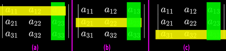
• Delete the row in which a₂₁ is situated. This is indicated by the yellow rectangle in fig,20.3(a) below:

Fig.20.3

• Delete the column in which a₂₁ is situated. This is indicated by the green rectangle in fig,20.3(a) above.
• Now write the following three items:
(i) The 2 × 2 determinant obtained by deleting the row and column.
(ii) Element which is under consideration. Here it is a₂₁.
(iii) (-1)^s, where s is the sum of the suffices of a₂₁.
So (-1)^s = (-1)²⁺¹.
• Finally, multiply the three items together. We get:
$(-1)^{2+1} \times a_{21} \times \left|\begin{array}{r}               
a_{12}    &{    a_{13}    }    \\
a_{32}    &{    a_{33}    }    \\
\end{array}\right|$   

Step 2:
• Take the second element of R₂, which is a₂₂.
• Delete the row in which a₂₂ is situated. This is indicated by the yellow rectangle in fig.20.3(b) above.
• Delete the column in which a₂₂ is situated. This is indicated by the green rectangle in fig.20.3(b) above.
• Now write the following three items:
(i) The 2 × 2 determinant obtained by deleting the row and column.
(ii) Element which is under consideration. Here it is a₂₂.
(iii) (-1)^s, where s is the sum of the suffices of a₂₂.
So (-1)^s = (-1)²⁺².
• Finally, multiply the three items together. We get:
$(-1)^{2+2} \times a_{22} \times \left|\begin{array}{r}               
a_{11}    &{    a_{13}    }    \\
a_{31}    &{    a_{33}    }    \\
\end{array}\right|$   

Step 3:
• Take the third element of R₂, which is a₂₃.
• Delete the row in which a₂₃ is situated. This is indicated by the yellow rectangle in fig,20.3(c) above.
• Delete the column in which a₂₃ is situated. This is indicated by the green rectangle in fig,20.3(c) above.
• Now write the following three items:
(i) The 2 × 2 determinant obtained by deleting the row and column.
(ii) Element which is under consideration. Here it is a₂₃.
(iii) (-1)^s, where s is the sum of the suffices of a₂₃.
So (-1)^s = (-1)²⁺³.
• Finally, multiply the three items together. We get:
$(-1)^{2+3} \times a_{23} \times \left|\begin{array}{r}               
a_{11}    &{    a_{12}    }    \\
a_{31}    &{    a_{32}    }    \\
\end{array}\right|$

Step 4:
• This is the final step. Here we add the results obtained in the above three steps.
• The sum thus obtained is the determinant of A. We can write:

◼ The process by which we apply the above four steps to find the determinant of order 3, is known as expansion along R₂.

---

• We saw two expansions:
   ♦ Expansion along R₁
   ♦ Expansion along R₂
Both gave the same result.

• In fact, there is a total of six expansions (corresponding to the three rows and three columns):
   ♦ Expansion along R₁
   ♦ Expansion along R₂
   ♦ Expansion along R₃
   ♦ Expansion along C₁
   ♦ Expansion along C₂
   ♦ Expansion along C₃

• All six will give the same result.

---

Let us try one more:

Expansion along C₃

Step 1:
• Take the first element of C₃, which is a₁₃.
• Delete the column in which a₁₃ is situated. This is indicated by the green rectangle in fig,20.4(a) below:

Fig.20.4

• Delete the row in which a₁₃ is situated. This is indicated by the yellow rectangle in fig,20.3(a) above.
• Now write the following three items:
(i) The 2 × 2 determinant obtained by deleting the column and row.
(ii) Element which is under consideration. Here it is a₁₃.
(iii) (-1)^s, where s is the sum of the suffices of a₁₃.
So (-1)^s = (-1)¹⁺³.
• Finally, multiply the three items together. We get:
$(-1)^{1+3} \times a_{13} \times \left|\begin{array}{r}               
a_{21}    &{    a_{22}    }    \\
a_{31}    &{    a_{32}    }    \\
\end{array}\right|$   

Step 2:
• Take the second element of C₃, which is a₂₃.
• Delete the column in which a₂₃ is situated. This is indicated by the green rectangle in fig,20.4(b) above.
• Delete the row in which a₂₃ is situated. This is indicated by the yellow rectangle in fig,20.4(b) above.
• Now write the following three items:
(i) The 2 × 2 determinant obtained by deleting the row and column.
(ii) Element which is under consideration. Here it is a₂₃.
(iii) (-1)^s, where s is the sum of the suffices of a₂₃.
So (-1)^s = (-1)²⁺³.
• Finally, multiply the three items together. We get:
$(-1)^{2+3} \times a_{23} \times \left|\begin{array}{r}               
a_{11}    &{    a_{12}    }    \\
a_{31}    &{    a_{32}    }    \\
\end{array}\right|$   

Step 3:
• Take the third element of C₃, which is a₃₃.
• Delete the column in which a₃₃ is situated. This is indicated by the green rectangle in fig,20.3(c) above.
• Delete the row in which a₃₃ is situated. This is indicated by the yellow rectangle in fig,20.3(c) above.
• Now write the following three items:
(i) The 2 × 2 determinant obtained by deleting the row and column.
(ii) Element which is under consideration. Here it is a₃₃.
(iii) (-1)^s, where s is the sum of the suffices of a₃₃.
So (-1)^s = (-1)³⁺³.
• Finally, multiply the three items together. We get:
$(-1)^{3+3} \times a_{33} \times \left|\begin{array}{r}               
a_{11}    &{    a_{12}    }    \\
a_{21}    &{    a_{22}    }    \\
\end{array}\right|$

Step 4:
• This is the final step. Here we add the results obtained in the above three steps.
• The sum thus obtained is the determinant of A. We can write:

◼ The process by which we apply the above four steps to find the determinant of order 3, is known as expansion along C₃.

---

• We saw three expansions:
   ♦ Expansion along R₁
   ♦ Expansion along R₂
   ♦ Expansion along C₃
All of then gave the same result.

• We can use any one of the six expansions that we mentioned earlier. The reader may write the 4 steps for R₃, C₁, C₂ and become convinced about this fact.

---

• Based on the above discussion, we can write two points:
(i) We must always use the expansion along that row/column which has the maximum number of zeroes.
(ii) Consider the term (-1)^s. Instead of calculating (-1)^s, we can put:
   ♦ 1 in the place of (-1)^s, if s is even   
   ♦ -1 in the place of (-1)^s, if s is odd.

---

Now we will see a special case. It can be written in steps:
1. Consider two matrices A = $\left[\begin{array}{r}        3    &{    3    }    \\
6    &{    0    }    \\
\end{array}\right]               
$ and B = $\left[\begin{array}{r}                
1    &{    1    }    \\
2    &{    0    }    \\
\end{array}\right]$               
 
• We see that A = 3B
2. Let us calculate the two determinants:
   ♦ |A| = 3(0) − 6(3) = −18
   ♦ |B| = 1(0) − 2(1) = −2
3. We see that:
|A| = 9(-2) = 3²|B|
• Note that, the exponent of 3 is 2. This 2 is the order of both A and B.
4. This can be written in general form as:
If A = kB, then |A| = kⁿ|B|, where n is the order of the two matrices A and B.
5. The formula written in (4) is applicable for the following three cases:
(i) When both A and B are matrices of order 1. 
(ii) When both A and B are matrices of order 2. 
(iii) When both A and B are matrices of order 3.

---

• We have seen the method for calculating determinant, when the given matrix is of the order 2 or 3.
• What about the determinant of a matrix, whose order is 1?
• Answer is simple:
For a 1 × 1 matrix [a], the determinant is a. 

---

In the next section, we will see some solved examples related to determinants.

Previous

Contents

Next

Copyright©2024 Higher secondary mathematics.blogspot.com

Chapter 20 - Determinants

In the previous section, we completed a discussion on matrices. In this chapter, we will see determinants.

Some basics about determinants can be written in 6 steps:
1. Consider any square matrix A.
• Using some simple steps, we can find a unique number related to that matrix.
• This number is called determinant of A.
2. Symbolically, we denote this number as |A|.
    ♦ It should not be read as modulus of A.
    ♦ It should be read as determinant of A.
3. There are two more ways for denoting this number:
   ♦ det(A)
   ♦ Δ
4. Let us see an example:
If $A = \left[\begin{array}{r}               
a    &{    b    }    \\
c    &{    d    }    \\
\end{array}\right]$, then $|A| ~=~ \left|\begin{array}{r}              
a    &{    b    }    \\
c    &{    d    }    \\
\end{array}\right|
~=~ \text{det}(A)$
 
5. Only square matrices have determinants.
6. The determinant can be a real number or a complex number.
• In this chapter we will be dealing with only those determinants, which are real numbers.

---

Method for finding the determinant of a 2 × 2 matrix

• This can be written in 3 steps:
1. Let A = $\left[\begin{array}{r}               
a_{11}    &{    a_{12}    }    \\
a_{21}    &{    a_{22}    }    \\
\end{array}\right]$
2. Then det(A) = |A| = $\left|\begin{array}{r}               
a_{11}    &{    a_{12}    }    \\
a_{21}    &{    a_{22}    }    \\
\end{array}\right|~=~a_{11}a_{22}~-~a_{21}a_{12}$
3. Note that, there are two terms in the determinant.
• Each term is a product of two elements, taken in a specified order. This order is indicated by the yellow arrows in fig.20.1 below:

Fig.20.1

• After calculating the two terms, we subtract the second term from the first.

---

Solved example 20.1
Evaluate $\left|\begin{array}{r}               
2    &{    4    }    \\
-1    &{    2    }    \\
\end{array}\right|$
Solution:
$\left|\begin{array}{r}               
2    &{    4    }    \\
-1    &{    2    }    \\
\end{array}\right|$ = 2(2) − 4(−1) = 4+4 = 8

Solved example 20.2
Evaluate $\left|\begin{array}{r}               
x    &{    x+1    }    \\
x-1    &{    x    }    \\
\end{array}\right|$
Solution:
$\begin{array}{ll} {~\color{magenta}    1    }    &{{}}    &{\left|\begin{array}{c}                x    &{    x+1    }    \\ x-1    &{    x    }    \\ \end{array}\right|}    & {~=~}    &{x(x)-(x+1)(x-1)}    \\
{~\color{magenta}    2    }    &{{}}    &{{}}    & {~=~}    &{x^2-(x^2 – 1)}    \\
{~\color{magenta}    3    }    &{{}}    &{{}}    & {~=~}    &{x^2- x^2 + 1}    \\
{~\color{magenta}    4    }    &{{}}    &{{}}    & {~=~}    &{1}    \\
\end{array}$

---

Method for finding the determinant of a 3 × 3 matrix

• Consider the 3 × 3 matrix A = $\left[\begin{array}{r}                           
a_{11}     &{    a_{12}     }    &{    a_{13}      }    \\
a_{21}      &{    a_{22}     }    &{    a_{23}      }    \\
a_{31}      &{    a_{32}       }    &{    a_{33}        }    \\
\end{array}\right]$
• We want $\left|\begin{array}{r}                           
a_{11}     &{    a_{12}     }    &{    a_{13}      }    \\
a_{21}      &{    a_{22}     }    &{    a_{23}      }    \\
a_{31}      &{    a_{32}       }    &{    a_{33}        }    \\
\end{array}\right|$
• Let us use the first row R₁. It can be done in 4 steps:
Step 1:
• Take the first element of R₁, which is a₁₁.
• Delete the row in which a₁₁ is situated.
• This is indicated by the yellow rectangle in fig,20.2(a) below:

Fig.20.2

• Delete the column in which a₁₁ is situated.
• This is indicated by the green rectangle in fig,20.2(a) above.
• Now write the following three items:
(i) The 2 × 2 determinant obtained by deleting the row and column.
(ii) Element which is under consideration. Here it is a₁₁.
(iii) (-1)^s, where s is the sum of the suffices of a₁₁.
So (-1)^s = (-1)¹⁺¹.
• Finally, multiply the three items together. We get:
$(-1)^{1+1} \times a_{11} \times \left|\begin{array}{r}               
a_{22}    &{    a_{23}    }    \\
a_{32}    &{    a_{33}    }    \\
\end{array}\right|$   

Step 2:
• Take the second element of R₁, which is a₁₂.
• Delete the row in which a₁₂ is situated.
• This is indicated by the yellow rectangle in fig,20.2(b) above.
• Delete the column in which a₁₂ is situated.
• This is indicated by the green rectangle in fig,20.2(b) above.
• Now write the following three items:
(i) The 2 × 2 determinant obtained by deleting the row and column.
(ii) Element which is under consideration. Here it is a₁₂.
(iii) (-1)^s, where s is the sum of the suffices of a₁₂.
So (-1)^s = (-1)¹⁺².
• Finally, multiply the three items together. We get:
$(-1)^{1+2} \times a_{12} \times \left|\begin{array}{r}               
a_{21}    &{    a_{23}    }    \\
a_{31}    &{    a_{33}    }    \\
\end{array}\right|$   

Step 3:
• Take the third element of R₁, which is a₁₃.
• Delete the row in which a₁₃ is situated.
• This is indicated by the yellow rectangle in fig,20.2(c) above.
• Delete the column in which a₁₃ is situated.
• This is indicated by the green rectangle in fig,20.2(c) above.
• Now write the following three items:
(i) The 2 × 2 determinant obtained by deleting the row and column.
(ii) Element which is under consideration. Here it is a₁₃.
(iii) (-1)^s, where s is the sum of the suffices of a₁₃.
So (-1)^s = (-1)¹⁺³.
• Finally, multiply the three items together. We get:
$(-1)^{1+3} \times a_{13} \times \left|\begin{array}{r}               
a_{21}    &{    a_{22}    }    \\
a_{31}    &{    a_{32}    }    \\
\end{array}\right|$

Step 4:
• This is the final step. Here we add the results obtained in the above three steps.
• The sum thus obtained is the determinant of A. We can write:

◼ The above process by which we apply the four steps to find the determinant of order 3, is known as expansion along R₁.

---

In the next section, we will see the process of finding the determinant by expansion along R₂.

Previous

Contents

Next

Copyright©2024 Higher secondary mathematics.blogspot.com

19.16 - Miscellaneous Examples

In the previous section, we completed a discussion on inverse matrix. In this section, we will see some miscellaneous examples.

Solved Example 19.19
If A = $\left[\begin{array}{r}               
\cos \theta     &{    \sin \theta    }    \\
-\sin \theta     &{    \cos \theta    }  \\
\end{array}\right]               
$, then prove that Aⁿ = $\left[\begin{array}{r}               
\cos n \theta     &{    \sin n \theta    }    \\
-\sin n \theta     &{    \cos n \theta    }  \\
\end{array}\right]               
$, where n is any natural number.
Solution:
We will prove this by using the principle of mathematical induction. Details can be seen here.

1. For any natural number, let P(n) denote the given statement. Then we can write:

P(n): If A = $\left[\begin{array}{r}               
\cos \theta     &{    \sin \theta    }    \\
-\sin \theta     &{    \cos \theta    }  \\
\end{array}\right]               
$, then Aⁿ = $\left[\begin{array}{r}               
\cos n \theta     &{    \sin n \theta    }    \\
-\sin n \theta     &{    \cos n \theta    }  \\
\end{array}\right]               
$

2. Basic step: (n=1)

• We see that, the statement is true when n = 1

3. Inductive step: (n=k) and (n= k+1)

(i) n = k

P(k): If A = $\left[\begin{array}{r}               
\cos \theta     &{    \sin \theta    }    \\
-\sin \theta     &{    \cos \theta    }  \\
\end{array}\right]               
$, then A^k = $\left[\begin{array}{r}               
\cos k \theta     &{    \sin k \theta    }    \\
-\sin k \theta     &{    \cos k \theta    }  \\
\end{array}\right]               
$

• We will assume that, this statement is true. 

(ii) n = k+1
• We need to prove the statement:
P(k+1): If A = $\left[\begin{array}{r}               
\cos \theta     &{    \sin \theta    }    \\
-\sin \theta     &{    \cos \theta    }  \\
\end{array}\right]               
$, then A^k+1 = $\left[\begin{array}{r}               
\cos (k+1) \theta     &{    \sin (k+1) \theta    }    \\
-\sin (k+1) \theta     &{    \cos (k+1) \theta    }  \\
\end{array}\right]               
$

• This can be proved as follows:

◼ Remarks:
In (2 magenta color), we are able to replace A^k. This is because, we assumed that, P(k) is true.

4. Thus P(k+1) is true whenever P(k) is true. Hence by the principle of mathematical induction, P(n) is true for any natural number n.

Solved Example 19.20
If A and B are symmetric matrices of the same order, then show that AB is symmetric if and only if A and B are commute, that is AB = BA
Solution:
1. If AB is to be symmetric, then it should be equal to it’s transpose. That is:
AB = (AB)'.
2. We know that, (AB)' = B'A'.
3. So the result in (1) becomes:
AB is symmetric if and only if AB = B'A'.
4. But given that, A and B are symmetric matrices. So we get:
A' = A and B' = B
5. So the result in (3) becomes:
AB is symmetric if and only if AB = BA.

---

• We can show the converse also:
AB = BA, if and only if AB is symmetric.
This can be shown in 3 steps:
1. If AB = BA, then we can write: AB = B'A'.
• This is because, A and B are said to be symmetric matrices. So A' = A and B' = B
2. We know that (AB)' = B'A'.
• So the result in (1) becomes:
If AB = BA, then AB = (AB)'.
3. But AB = (AB)' indicates that, AB is symmetric.
• So the result in (2) becomes:
If AB = BA, then AB is symmetric.

Solved Example 19.21
Let $A = \left[\begin{array}{r}               
2     &{    -1    }    \\
3     &{    4    }  \\
\end{array}\right] ,~ B = \left[\begin{array}{r}               
5     &{    2    }    \\
7     &{    4    }  \\
\end{array}\right],~ C = \left[\begin{array}{r}               
2     &{    5    }    \\
3     &{    8    }  \\
\end{array}\right]$.
Find a matrix D such that CD – AB = O
Solution:
1. Finding the order of D:
• Both A and B are 2 × 2 matrices. So AB will be a 2 × 2 matrix.
• AB is being subtracted from CD. So CD will be a 2 × 2 matrix.
• In CD, the matrix C is a 2 × 2 matrix. So we have two points:
    ♦ CD is a 2 × 2 matrix.
    ♦ C is a 2 × 2 matrix.
• Let D be of the order m × n.
• Comparing the orders of C and D to form CD, we see that:
    ♦ m must be 2
    ♦ n must be 2
• So the order of D is 2 × 2

2. Let $D = \left[\begin{array}{r}               
a     &{    b    }    \\
c     &{    d    }  \\
\end{array}\right]$.

3. Given that, CD – AB = O
This can be rearranged as shown below:

◼ Remarks:
Magenta 2: We add AB on both sides.

4. By equality of matrices, we get four equations:
(i) 2a + 5c = 3
(ii) 2b + 5d = 0
(iii) 3a + 8c = 43
(iv) 3b + 8d = 22

5. Now we can solve the equations:
• Solving (i) and (iii), we get: a = -191 and c = 77
• Solving (ii) and (iv), we get: b = -110 and d = 44

6. So the required matrix can be written as:
$D = \left[\begin{array}{r}               
a     &{    b    }    \\
c     &{    d    }  \\
\end{array}\right] ~=~ \left[\begin{array}{r}               
-191     &{    -110    }    \\
77     &{    44    }  \\
\end{array}\right]$.

Alternate method:
Since all matrices involved are square matrices, we can apply inverse.

1. Given that, CD – AB = O
This can be rearranged as shown below:

◼ Remarks:
Magenta 2: We add AB on both sides.
Magenta 4: We pre multiply both sides by C^-1.

2. So our next task is to find C^-1.

3. Our next task is to find AB:

4. Our final task is to find D:

---

The link below gives a few more examples:

Miscellaneous Exercise

---

In the next chapter, we will see Determinants.

Previous

Contents

Next 

Copyright©2024 Higher secondary mathematics.blogspot.com

19.15 - Solved Examples

In the previous section, we saw a method to find the inverse of a given matrix. We saw a solved example also. In this section, we will see a few more solved examples.

Let us see some solved examples:

Solved Example 19.17
By using elementary operations, find the inverse of the matrix A = $\left[\begin{array}{r}               
0    &{    1    } &{    2    }    \\
1    &{    2    }  &{    3    }  \\
3    &{    1    }  &{    1    }  \\
\end{array}\right]               
$
Solution:
Method 1: Using elementary row operations.
• We can write a general procedure:
1. We are given a 3×3 matrix.
• So the diagonal elements are: a₁₁, a₂₂ and a₃₃. These elements must be ‘1’ in the final answer.
2. First we change a₁₁ to 1.
• Then we change the remaining elements in that column, to zeros. We do that step by step.
3. Next, we change a₂₂ to 1.
• Then we change the remaining elements in that column, to zeros. We do that step by step.
4. Finally, we change a₃₃ to 1.
• Then we change the remaining elements in that column, to zeros. We do that step by step.

Method 2: Using elementary column operations.
• We can write a general procedure:
1. We are given a 3×3 matrix.
• So the diagonal elements are: a₁₁, a₂₂ and a₃₃. These elements must be ‘1’ in the final answer.
2. First we change a₁₁ to 1.
• Then we change the remaining elements in that row, to zeros. We do that step by step.
3. Next, we change a₂₂ to 1.
• Then we change the remaining elements in that row, to zeros. We do that step by step.
4. Finally, we change a₃₃ to 1.
• Then we change the remaining elements in that row, to zeros. We do that step by step.

Solved Example 19.18
By using elementary operations, find the inverse of the matrix A = $\left[\begin{array}{r}               
10    &{    -2    }    \\
-5    &{    1    }    \\
\end{array}\right]               
$
Solution:
Method 1: Using elementary row operations.

• We see that:
In (4) we did an elementary operation. As a result of that single operation, all elements of a row became zeroes.
• So for the given matrix A, the inverse does not exist.

---

The link below gives a few more solved examples:

Exercise 19.4

---

In the next section, we will see some miscellaneous examples.

Previous

Contents

Next

Copyright©2024 Higher secondary mathematics.blogspot.com

19.14 - Finding the Inverse Matrix

In the previous section, we saw the basics of invertible matrices. In this section, we will see the two theorems related to invertible matrices. Later in this section, we will see the method to find the inverse of a given matrix.

Theorem 1:
There will be only one inverse matrix.
• The proof can be written in 8 steps:
1. Let A be a square matrix. Let us assume that, B and C are inverse matrices of A.
2. Since B is an inverse of A, we can write: AB = BA = I
3. Since C is an inverse of A, we can write: AC = CA = I
4. Any matrix multiplied by I will give the same matrix. So we have: B = BI
5. But from (3), we have: I = AC
• So the result in (4) becomes: B = BI = B(AC)
6. Recall the associative law: X(YZ) = (XY)Z (Details here)
• Applying the law, the result in (5) becomes:
B = BI = B(AC) = (BA)C
7. But from (2), we have: BA = I
• So the result in (6) becomes:
B = BI = B(AC) = (BA)C = IC = C
8. Thus we get B = C
That means, there can be only one inverse.

Theorem 2
If A and B are invertible matrices of the same order, then (AB)^-1 = B^-1A^-1.
• Proof can be written in steps:
1. We know that (X)(X)^-1 = I
So we can write: (AB)(AB)^-1 = I
2. Pre multiplying both sides by A^-1, we get:
A^-1(AB)(AB)^-1 = A^-1I
⇒ A^-1(AB)(AB)^-1 = A^-1
3. Applying associative law, we get:
(A^-1A)B(AB)^-1 = A^-1.
⇒ IB(AB)^-1 = A^-1.
⇒ B(AB)^-1 = A^-1.
4. Pre multiplying both sides by B^-1, we get:
B^-1B(AB)^-1 = B^-1A^-1.
⇒ I(AB)^-1 = B^-1A^-1.
⇒ (AB)^-1 = B^-1A^-1.

---

Inverse of a Matrix by elementary operations

First we will see how elementary operations can be applied to a matrix equation. It can be written in 3 steps:
1. Consider the equation: X = AB, where X, A and B are square matrices of the same order.
2. We can perform elementary operations on this equation.
• But while performing the operations, the equality should be maintained.
3. For maintaining the equality, we follow a procedure:
• Whatever elementary row operation is performed on the L.H.S, the same operation must be performed on the first matrix A on the R.H.S.
• Whatever elementary column operation is performed on the L.H.S, the same operation must be performed on the second matrix B on the R.H.S.

---

The above steps give us a method to find the inverse of a matrix. It can be written in 3 steps:
1. Consider the equation A = IA
• We can perform a series of elementary row operations on this equation, till we reach the form: I = BA
• So our aim is to transform A on the L.H.S to I
• Based on step (3), we can say that, A on the L.H.S, and I on the R.H.S will get transformed during the process.
    ♦ A in the L.H.S will become I.
    ♦ I in the R.H.S will become B.
• Once we get I = BA, it implies that, B is the inverse of A.
2. There is an alternate method to find the inverse.
• Consider the equation A = AI
• We can perform a series of elementary column operations on this equation, till we reach the form: I = AB
• So here also, our aim is to transform A on the L.H.S to I
• Based on step (3), we can say that, A on the L.H.S, and I on the R.H.S will get transformed during the process.
    ♦ A in the L.H.S will become I.
    ♦ I in the R.H.S will become B.
• Once we get I = AB, it implies that, B is the inverse of A.
3. Let us compare the two methods:
(i) Use of elementary operations:
    ♦ In (1), we use elementary row operations.
    ♦ In (2), we use elementary column operations.
(ii) Initial equation:
    ♦ In (1), the initial equation is A = IA
    ♦ In (2), the initial equation is A = AI
(iii) Final equation:
    ♦ In (1), the final equation is I = BA
    ♦ In (2), the final equation is I = AB
(iv) In both (1) and (2),
    ♦ A on the L.H.S is transformed into I.
    ♦ I on the R.H.S is transformed into B.

---

Let us see a solved example:

Solved Example 19.16
By using elementary operations, find the inverse of the matrix A = $\left[\begin{array}{r}               
1    &{    2    }    \\
2    &{    -1    }    \\
\end{array}\right]               
$
Solution:
Method 1: Using elementary row operations.
• We can write a general procedure:
1. We are given a 2×2 matrix.
• So the diagonal elements are: a₁₁ and a₂₂. These elements must be ‘1’ in the final answer.
2. First we change a₁₁ to 1.
• Then we change the remaining elements in that column, to zeros. We do that step by step.
3. Next, we change a₂₂ to 1.
• Then we change the remaining elements in that column, to zeros. We do that step by step.

$\begin{array}{ll} {~\color{magenta}    1    }    &{{}}    &{A}    & {~=~}    &{IA}    \\
{~\color{magenta}    2    }    &{\implies}    &{\left[\begin{array}{r}



1
&{
2
}
\\ 2
&{
-1
}
\\ \end{array}\right]



}    & {~=~}    &{\left[\begin{array}{r}



1
&{
0
}
\\ 0
&{
1
}
\\ \end{array}\right]A }    \\
{~\color{magenta}    3    }    &{R_2 \rightarrow {R_2 \;–\; 2 R_1}}    &{\left[\begin{array}{r}



1
&{
2
}
\\ 0
&{
-5
}
\\ \end{array}\right]



}    & {~=~}    &{\left[\begin{array}{r}



1
&{
0
}
\\ -2
&{
1
}
\\ \end{array}\right]



A}    \\
{~\color{magenta}    4    }    &{R_2 \rightarrow {-\frac{1}{5} R_2}}    &{\left[\begin{array}{r}



1
&{
2
}
\\ 0
&{
1
}
\\ \end{array}\right]



}    & {~=~}    &{\left[\begin{array}{r}



1
&{
0
}
\\ \frac{2}{5}
&{
-\frac{1}{5}
}
\\ \end{array}\right]



A}    \\
{~\color{magenta}    5    }    &{R_1 \rightarrow {R_1 \,–\, 2 R_2}}    &{\left[\begin{array}{r}



1
&{
0
}
\\ 0
&{
1
}
\\ \end{array}\right]



}    & {~=~}    &{\left[\begin{array}{r}



\frac{1}{5}
&{
\frac{2}{5}
}
\\ \frac{2}{5}
&{
-\frac{1}{5}
}
\\ \end{array}\right]



A}    \\
{~\color{magenta}    6    }    &{\implies}    &{I}    & {~=~}    &{\left[\begin{array}{r}



\frac{1}{5}
&{
\frac{2}{5}
}
\\ \frac{2}{5}
&{
-\frac{1}{5}
}
\\ \end{array}\right]



A}    \\
{~\color{magenta}    7    }    &{~\text{But}}    &{I}    & {~=~}    &{A^{-1} A}    \\
{~\color{magenta}    8    }    &{\implies}    &{A^{-1}}    & {~=~}    &{\left[\begin{array}{r}



\frac{1}{5}
&{
\frac{2}{5}
}
\\ \frac{2}{5}
&{
-\frac{1}{5}
}
\\ \end{array}\right]



}    \\
\end{array}$

◼ Remarks:
• a₁₁ is already ‘1’.
    ♦ The remaining element in that column is a₂₁.
    ♦ We must change it to zero. This is achieved in (3).
• a₂₂ is changed to ‘1’ in (4).
    ♦ The remaining element in that column is a₁₂.
    ♦ We must change it to zero. This is achieved in (5).

Method 2: Using elementary column operations.
• We can write a general procedure:
1. We are given a 2×2 matrix.
• So the diagonal elements are: a₁₁ and a₂₂. These elements must be ‘1’ in the final answer.
2. First we change a₁₁ to 1.
• Then we change the remaining elements in that row, to zeros. We do that step by step.
3. Next, we change a₂₂ to 1.
• Then we change the remaining elements in that row, to zeros. We do that step by step.

$\begin{array}{ll} {~\color{magenta}    1    }    &{{}}    &{A}    & {~=~}    &{AI}    \\
{~\color{magenta}    2    }    &{\implies}    &{\left[\begin{array}{r}



1
&{
2
}
\\ 2
&{
-1
}
\\ \end{array}\right]



}    & {~=~}    &{A \left[\begin{array}{r}



1
&{
0
}
\\ 0
&{
1
}
\\ \end{array}\right]}    \\
{~\color{magenta}    3    }    &{C_2 \rightarrow {C_2 \;–\; 2 C_1}}    &{\left[\begin{array}{r}



1
&{
0
}
\\ 2
&{
-5
}
\\ \end{array}\right]



}    & {~=~}    &{A \left[\begin{array}{r}



1
&{
-2
}
\\ 0
&{
1
}
\\ \end{array}\right]



}    \\
{~\color{magenta}    4    }    &{C_2 \rightarrow {-\frac{1}{5} C_2}}    &{\left[\begin{array}{r}



1
&{
0
}
\\ 2
&{
1
}
\\ \end{array}\right]







}    & {~=~}    &{A





\left[\begin{array}{r}



1
&{
\frac{2}{5}
}
\\ 0
&{
-\frac{1}{5}
}
\\ \end{array}\right]



}    \\
{~\color{magenta}    5    }    &{C_1 \rightarrow {C_1 \,–\, 2 C_2}}    &{\left[\begin{array}{r}



1
&{
0
}
\\ 0
&{
1
}
\\ \end{array}\right]







}    & {~=~}    &{A






\left[\begin{array}{r}



\frac{1}{5}
&{
\frac{2}{5}
}
\\ \frac{2}{5}
&{
-\frac{1}{5}
}
\\ \end{array}\right]



}    \\
{~\color{magenta}    6    }    &{\implies}    &{I}    & {~=~}    &{A \left[\begin{array}{r}



\frac{1}{5}
&{
\frac{2}{5}
}
\\ \frac{2}{5}
&{
-\frac{1}{5}
}
\\ \end{array}\right]



}    \\
{~\color{magenta}    7    }    &{~\text{But}}    &{I}    & {~=~}    &{A A^{-1} }    \\
{~\color{magenta}    8    }    &{\implies}    &{A^{-1}}    & {~=~}    &{\left[\begin{array}{r}



\frac{1}{5}
&{
\frac{2}{5}
}
\\ \frac{2}{5}
&{
-\frac{1}{5}
}
\\ \end{array}\right]



}    \\
\end{array}$

◼ Remarks:
• a₁₁ is already ‘1’.
    ♦ The remaining element in that column is a₁₂.
    ♦ We must change it to zero. This is achieved in (3).
• a₂₂ is changed to ‘1’ in (4).
    ♦ The remaining element in that row is a₂₁.
    ♦ We must change it to zero. This is achieved in (5).

---

In the next section, we will see a few more solved examples.

Previous

Contents

Next

Copyright©2024 Higher secondary mathematics.blogspot.com

19.13 - Invertible Matrices

In the previous section, we completed a discussion on symmetric and skew symmetric matrices. In this section, we will see elementary operations. Later in this section, we will see invertible matrices also.

Elementary Operation of a Matrix

• There are six operations on a matrix.
    ♦ They are known as elementary operations.
    ♦ They are also known as transformations.

Operation I:
This can be explained in 2 steps:
1. First pick two suitable rows. They need not be adjacent rows. Then interchange those two rows.
• For example, suppose that, we pick the first and third rows. After the operation, we will get a new matrix such that:
    ♦ First row in the original matrix, is the third row in the new matrix.
    ♦ Third row in the original matrix, is the first row in the new matrix.
2. Symbolically, we write this operation as: $R_i \leftrightarrow  R_j$.
• The example operation that we saw above, can be written symbolically as follows:
Applying $R_1 \leftrightarrow  R_3$ to $\left[\begin{array}{r}                           
3    &{    -10    }    &{    8    }    \\
11    &{    -4    }    &{    -9    }    \\
2    &{    12    }    &{    13    }    \\
\end{array}\right]                           
$, gives $\left[\begin{array}{r}                            
2    &{    12    }    &{    13    }    \\
11    &{    -4    }    &{    -9    }    \\
3    &{    -10    }    &{    8    }    \\
\end{array}\right]$.

Operation II:
This can be explained in 2 steps:
1. First pick a single suitable row. Then multiply each element of that row by a non zero number k.
• For example, suppose that, we pick the second row. After the operation, we will get a new matrix such that:
Each element in the second row is k times the original element.
2. Symbolically, we write this operation as: $R_i \rightarrow  k R_i$.
• The example operation that we saw above, can be written symbolically as follows:
Applying $R_2 \rightarrow  3 R_2$ to $\left[\begin{array}{r}                           
3    &{    -10    }    &{    8    }    \\
11    &{    -4    }    &{    -9    }    \\
2    &{    12    }    &{    13    }    \\
\end{array}\right]                           
$, gives $\left[\begin{array}{r}                            
3    &{    -10    }    &{    8    }    \\
33    &{    -12    }    &{    -27    }    \\
2    &{    12    }    &{    13    }    \\
\end{array}\right]$.

Operation III:
This can be explained in 2 steps:
1. First pick a single suitable row. Then multiply each element of that row by a non zero number k. Finally, add each member of the new row with the corresponding element of another suitable row.
2. Symbolically, we write this operation as: $R_i \rightarrow  R_i + k R_j$.
• Let us see an example:
Applying $R_3 \rightarrow  R_3 - 2 R_1$ to $\left[\begin{array}{r}                           
3    &{    -10    }    &{    8    }    \\
11    &{    -4    }    &{    -9    }    \\
2    &{    12    }    &{    13    }    \\
\end{array}\right]                           
$, gives $\left[\begin{array}{r}                            
3    &{    -10    }    &{    8    }    \\
11    &{    -4    }    &{    -9    }    \\
-4    &{    32    }    &{    -3    }    \\
\end{array}\right]$.

Operation IV:
• This is similar to the operation I. Instead of rows, we deal with columns.
• An example:
Applying $C_2 \leftrightarrow  C_3$ to $\left[\begin{array}{r}                           
3    &{    -10    }    &{    8    }    \\
11    &{    -4    }    &{    -9    }    \\
2    &{    12    }    &{    13    }    \\
\end{array}\right]                           
$, gives $\left[\begin{array}{r}                           
3    &{    8    }    &{    -10    }    \\
11    &{    -9    }    &{    -4    }    \\
2    &{    13    }    &{    12    }    \\
\end{array}\right]                           
$.

Operation V:
• This is similar to the operation II. Instead of rows, we deal with columns.
• An example:
Applying $C_3 \rightarrow  2C_3$ to $\left[\begin{array}{r}                           
3    &{    -10    }    &{    8    }    \\
11    &{    -4    }    &{    -9    }    \\
2    &{    12    }    &{    13    }    \\
\end{array}\right]                           
$, gives $\left[\begin{array}{r}                           
3    &{    -10    }    &{    16    }    \\
11    &{    -4    }    &{    -18    }    \\
2    &{    12    }    &{    26    }    \\
\end{array}\right]                           
$.

Operation VI:
• This is similar to the operation III. Instead of rows, we deal with columns.
• An example:
Applying $C_1 \rightarrow  C_1 + 1.5 C_2$ to $\left[\begin{array}{r}                           
3    &{    -10    }    &{    8    }    \\
11    &{    -4    }    &{    -9    }    \\
2    &{    12    }    &{    13    }    \\
\end{array}\right]                           
$, gives $\left[\begin{array}{r}                           
-12    &{    -10    }    &{    8    }    \\
5    &{    -4    }    &{    -9    }    \\
20    &{    12    }    &{    13    }    \\
\end{array}\right]                           
$.

---

Invertible Matrices

This can be explained in 5 steps:
1. Consider two matrices A and B.
2. Suppose that, A and B satisfy three conditions:
(i) Both A and B are square matrices.
(ii) Both A and B are of the same order m.
(iii) AB = BA = I
3. If the three conditions are satisfied, then:
• B is called the inverse matrix of A.
    ♦ The inverse matrix of A is denoted as A^-1.
    ♦ So B = A^-1.
• A is called the inverse matrix of B.
    ♦ The inverse matrix of B is denoted as B^-1.
    ♦ So A = B^-1.
4. If it is possible to find A^-1, then we say that:
A is an invertible matrix.
5. An example is shown below:

• In the above example, we can write:
    ♦ AB = BA = I
    ♦ B is the inverse of A. In other words, B = A^-1.
    ♦ A is the inverse of B. In other words, A = B^-1.
    ♦ A is an invertible matrix.
    ♦ B is an invertible matrix.

---

Note:
A rectangular matrix will not have an inverse. This can be demonstrated using an example. It can be written in 6 steps:
1. Suppose that, A is a rectangular matrix, of order 2 × 3
2. Let B be the inverse of A
Then AB = BA
3. If A is to be multiplied by B, then a possible order of B is: 3 × 2
• In that case, the order of AB will be 2 × 2.
4. The order of BA will be 3 × 3.
5. So we get:
    ♦ Order of AB = 2 × 2
    ♦ Order of BA = 3 × 3
• In such a situation, AB cannot be equal to BA.
• So B cannot be the inverse of A.
6. We can write:
Both A and B must be square matrices and both should be of the same order.

---

In the next section, we will see theorems related to invertible matrices.

Previous

Contents

Next

Copyright©2024 Higher secondary mathematics.blogspot.com

19.12 - Second Theorem

In the previous section, we saw the theorem 1 related to symmetric and skew symmetric matrices. In this section, we will see theorem 2.

Theorem 2
Any square matrix can be expressed as the sum of a symmetric matrix and a skew symmetric matrix.

Proof:
Let A be a square matrix. First, we will prove that,
$A = \frac{1}{2} \left(A + A' \right)~+~\frac{1}{2} \left(A - A' \right)$

$\begin{array}{ll} {~\color{magenta}    1    }    &{{}}    &{{}}    &{{}}    &{\frac{1}{2} \left(A + A' \right)~+~\frac{1}{2} \left(A - A' \right)}    \\
{~\color{magenta}    2    }    &{{}}    &{{}}    & {~=~}    &{\frac{1}{2} A ~+~\frac{1}{2} A' ~+~\frac{1}{2} A ~-~\frac{1}{2} A'}    \\
{~\color{magenta}    3    }    &{{}}    &{{}}    & {~=~}    &{\frac{1}{2} A ~+~\frac{1}{2} A ~+~\frac{1}{2} A' ~-~\frac{1}{2} A'}    \\
{~\color{magenta}    4    }    &{{}}    &{{}}    & {~=~}    &{\frac{1}{2} A ~+~\frac{1}{2} A}    \\
{~\color{magenta}    5    }    &{{}}    &{{}}    & {~=~}    &{A}    \\
\end{array}$

• Now we can write the proof for theorem 2 in  steps:
1. We just proved that, A can be written as the sum of two terms. $\frac{1}{2} \left(A + A' \right)$ and $\frac{1}{2} \left(A - A' \right)$
2. Consider the first term.
• In this term, we know (from theorem 1) that, (A+A') is a symmetric matrix.
• We need to prove that, $\frac{1}{2} \left(A + A' \right)$ is also a symmetric matrix.
• For that, we need to prove:
$\frac{1}{2} \left(A + A' \right)~=~\left[\frac{1}{2} \left(A + A' \right) \right]'$
• In other words, we need to prove:
$\frac{1}{2} B~=~\left[\frac{1}{2} B \right]'$
   ♦ Where B = A + A'
• This can be proved in 4 steps:
(i) B is symmetric.
   ♦ That means, B = B'
   ♦ That means, $\frac{1}{2} B ~=~ \frac{1}{2} B'$
(ii) For any matrix X, we have: kX' = (kX)'
(iii) So the result in (i) becomes:
$\frac{1}{2} B ~=~ \frac{1}{2} B' ~=~\left[\frac{1}{2} B \right]'$
(iv) By picking the first and last terms in (iii), we get:
$\frac{1}{2} B ~=~\left[\frac{1}{2} B \right]'$.
• This is same as:
$\frac{1}{2} \left(A + A' \right)~=~\left[\frac{1}{2} \left(A + A' \right) \right]'$
• So $\frac{1}{2} \left(A + A' \right)$ is a symmetric matrix.

3. Consider the second term.
• In this term, we know (from theorem 1) that, (A−A') is a skew symmetric matrix.
• We need to prove that, $\frac{1}{2} \left(A - A' \right)$ is also a skew symmetric matrix.
• For that, we need to prove:
$\frac{1}{2} \left(A - A' \right)~=~- \left[\frac{1}{2} \left(A - A' \right) \right]'$
• In other words, we need to prove:
$\frac{1}{2} C~=~- \left[\frac{1}{2} C \right]'$
   ♦ Where C = A − A'
• This can be proved in 4 steps:
(i) C is skew symmetric.
   ♦ That means, C = -C'
   ♦ That means, $\frac{1}{2} C ~=~ -\frac{1}{2} C'$
(ii) For any matrix X, we have: kX' = (kX)'
(iii) So the result in (i) becomes:
$\frac{1}{2} C ~=~ -\frac{1}{2} C' ~=~- \left[\frac{1}{2} C \right]'$
(iv) By picking the first and last terms in (iii), we get:
$\frac{1}{2} C ~=~-\left[\frac{1}{2} C \right]'$.
• This is same as:
$\frac{1}{2} \left(A - A' \right)~=~- \left[\frac{1}{2} \left(A - A' \right) \right]'$
• So $\frac{1}{2} \left(A - A' \right)$ is a skew symmetric matrix.

4. So the first term is a symmetric matrix. Also, the second term is a skew symmetric matrix.
• Thus we effectively wrote matrix A as the sum of a symmetric matrix and a skew symmetric matrix.
• Theorem 2 is proved.

---

Solved example 19.15
Express the matrix B = $\left[\begin{array}{r}                           
3    &{    11    }    &{    2    }    \\
-10    &{    -4    }    &{    12    }    \\
8    &{    -9    }    &{    13    }    \\
\end{array}\right]                           
$ as the sum of a symmetric matrix and a skew symmetric matrix.
Solution:
1. Write the transpose of B:
B' = $\left[\begin{array}{r}                           
3    &{    -10    }    &{    8    }    \\
11    &{    -4    }    &{    -9    }    \\
2    &{    12    }    &{    13    }    \\
\end{array}\right]                           
$

2. Let $P = \frac{1}{2} (B+B')$ and $Q = \frac{1}{2} (B-B')$

3. Finding P and proving that, it is symmetric:

• If we try to write P', we will get the same P. So P is a symmetric matrix.

4. Finding Q and proving that, it is skew symmetric:

 

• We see that, Q' = -Q. So it is a skew symmetric matrix.

5. Checking the sum:

---

The link below gives a few more solved examples:

Exercise 19.3

---

In the next section, we will see elementary operation of a matrix and invertible matrices.

Previous

Contents

Next

Copyright©2024 Higher secondary mathematics.blogspot.com