Chapter 13.14 - Graph of Derivatives

In the previous section, we saw the general form of the derivative. We saw some solved examples also. In this section, we will see a few more solved examples. We will also see the graphs of derivatives.

Solved example 13.10
Find the derivative of f(x) = 10x.
Solution:
• In our present case, f(x) = 10x. So we get:
$\begin{array}{ll}
{}&{f'(x)}
& {~=~}& {\lim_{h\rightarrow 0}{\left[\frac{f(x+h) – f(x)}{h} \right]}}
&{} \\

{}&{}
& {~=~}& {\lim_{h\rightarrow 0}{\left[\frac{10(x+h) – 10 x}{h} \right]}}
&{} \\

{}&{}
& {~=~}& {\lim_{h\rightarrow 0}{\left[\frac{10x + 10h – 10x}{h} \right]}}
&{} \\

{}&{}
& {~=~}& {\lim_{h\rightarrow 0}{\left[\frac{10h}{h} \right]}}
&{} \\

{}&{}
& {~=~}& {10 \lim_{h\rightarrow 0}{\left[\frac{h}{h} \right]}}
&{} \\

{}&{}
& {~=~}& {10 \lim_{h\rightarrow 0}{1}}
&{} \\

{}&{}
& {~=~}& {10 × 1}
&{} \\

{}&{}
& {~=~}& {10}
&{} \\

\end{array}$

◼ A graphical description can be written in 5 steps:
1. In the previous section, we saw that, f’(x) is a function. So we must  be able to plot f’(x).
2. In fig.13.34 below, both f(x) and f’(x) are plotted in the same graph.

Fig.13.34

• In order to accommodate both functions in the same graph, the scale is changed to the following values:
    ♦ x-axis: 1 unit = 2
    ♦ y-axis: 1 unit = 10
3. The two graphs are plotted in different colors.
    ♦ The red line represents f(x)
    ♦ The green line represents f’(x)
4. f’(x) is a constant function. So, as expected, the green line is horizontal.
5. Let us see the practical application of the graph. It can be written using two examples:
(i) Suppose that, we want the derivative of f(x) at (x = 1.5). That is., we want f’(1.5)
• For that, we mark point A on the red line. Here, (x = 1.5)
• Next we draw a vertical line through A. This vertical line meets the green line at A'.
• f’(1.5) will be equal to the y-coordinate of A'.
(ii) Suppose that, we want the derivative of f(x) at (x = -2.3). That is., we want f’(-2.3)
• For that, we mark point B on the red line. Here, (x = -2.3)
• Next we draw a vertical line through B. This vertical line meets the green line at B'.
• f’(-2.3) will be equal to the y-coordinate of B'.

Solved example 13.11
Find the derivative of f(x) = x² .
Solution:
• In our present case, f(x) = x². So we get:
$\begin{array}{ll}
{}&{f'(x)}
& {~=~}& {\lim_{h\rightarrow 0}{\left[\frac{f(x+h) – f(x)}{h} \right]}}
&{} \\

{}&{}
& {~=~}& {\lim_{h\rightarrow 0}{\left[\frac{[(x+h)^2] – [x^2]}{h} \right]}}
&{} \\

{}&{}
& {~=~}& {\lim_{h\rightarrow 0}{\left[\frac{[(x^2 + 2hx + h^2)] – [x^2]}{h} \right]}}
&{} \\

{}&{}
& {~=~}& {\lim_{h\rightarrow 0}{\left[\frac{2hx + h^2}{h} \right]}}
&{} \\

{}&{}
& {~=~}& {\lim_{h\rightarrow 0}{\left[\frac{h(h +2x)}{h} \right]}}
&{} \\

{}&{}
& {~=~}& {\lim_{h\rightarrow 0}{[h + 2x]}}
&{} \\

{}&{}
& {~=~}& {2x}
&{} \\

\end{array}$

◼ A graphical description can be written in 5 steps:
1. In the previous section, we saw that, f’(x) is a function. So we must  be able to plot f’(x).
2. In fig.13.35 below, both f(x) and f’(x) are plotted in the same graph.

Fig.13.35

3. The two graphs are plotted in different colors.
    ♦ The red curve represents f(x)
    ♦ The green line represents f’(x)
4. Let us see the practical application of the graph. It can be written using two examples:
(i) Suppose that, we want the derivative of f(x) at (x = 3). That is., we want f’(3)
• For that, we mark point A on the red line. Here, (x = 3)
• Next we draw a vertical line through A. This vertical line meets the green line at A'.
• f’(3) will be equal to the y-coordinate of A'. In this case, it is 6.
• We can verify this theoretically:
f`(3) = 2 × 3 = 6
(ii) Suppose that, we want the derivative of f(x) at (x = -2.5). That is., we want f’(-2.5)
• For that, we mark point B on the red line. Here, (x = -2.5)
• Next we draw a vertical line through B. This vertical line meets the green line at B'.
• f’(-2.5) will be equal to the y-coordinate of B'. In this case, it is -5.
• We can verify this theoretically:
f`(-2.5) = 2 × -2.5 = -5
5. Further more, the reader may verify the tangents also:
• Through the point A, draw a line at a slope of 6. This line will be tangential to f(x).
• Through the point B, draw a line at a slope of -5. This line will be tangential to f(x). 

Solved example 13.12
Find the derivative of the constant function f(x) = a for a fixed real number a.
Solution:
• In our present case, f(x) = a. So we get:

$\begin{array}{ll}
{}&{f'(x)}
& {~=~}& {\lim_{h\rightarrow 0}{\left[\frac{f(x+h) – f(x)}{h} \right]}}
&{} \\

{}&{}
& {~=~}& {\lim_{h\rightarrow 0}{\left[\frac{[a] – [a]}{h} \right]}}
&{} \\

{}&{}
& {~=~}& {\lim_{h\rightarrow 0}{\left[\frac{0}{h} \right]}}
&{} \\

{}&{}
& {~=~}& {0}
&{} \\

\end{array}$

Solved example 13.13
Find the derivative of f(x) = $\frac{1}{x}$.
Solution:
• In our present case, f(x) = $\frac{1}{x}$. So we get:
$\begin{array}{ll}
{}&{f'(x)}
& {~=~}& {\lim_{h\rightarrow 0}{\left[\frac{f(x+h) – f(x)}{h} \right]}}
&{} \\

{}&{}
& {~=~}& {\lim_{h\rightarrow 0}{\left[\frac{\left[\frac{1}{x+h}\right] – \left[\frac{1}{x}\right]}{h} \right]}}
&{} \\

{}&{}
& {~=~}& {\lim_{h\rightarrow 0}{\left[\frac{\frac{x - x - h}{x(x+h)}}{h} \right]}}
&{} \\

{}&{}
& {~=~}& {\lim_{h\rightarrow 0}{\left[\frac{-h}{xh(x+h)} \right]}}
&{} \\

{}&{}
& {~=~}& {\lim_{h\rightarrow 0}{\left[\frac{-1}{x(x+h)} \right]}}
&{} \\

{}&{}
& {~=~}& {\frac{-1}{x(x+0)}}
&{} \\

{}&{}
& {~=~}& {-\frac{1}{x^2}}
&{} \\

\end{array}$

◼ A graphical description can be written in 5 steps:
1. In the previous section, we saw that, f’(x) is a function. So we must  be able to plot f’(x).
2. In fig.13.36 below, both f(x) and f’(x) are plotted in the same graph.

Fig.13.36

3. The two graphs are plotted in different colors.
    ♦ The red curve represents f(x)
    ♦ The green curve represents f’(x)
4. Let us see the practical application of the graph. It can be written using two examples:
(i) Suppose that, we want the derivative of f(x) at (x = 1.5). That is., we want f’(1.5)
• For that, we mark point A on the red line. Here, (x = 1.5)
• Next we draw a vertical line through A. This vertical line meets the green line at A'.
• f’(1.5) will be equal to the y-coordinate of A'. In this case, it is -0.44.
• We can verify this theoretically:
f`(1.5) = $-\frac{1}{1.5^2}$ = -0.44
(ii) Suppose that, we want the derivative of f(x) at (x = -2). That is., we want f’(-2)
• For that, we mark point B on the red line. Here, (x = -2)
• Next we draw a vertical line through B. This vertical line meets the green line at B'.
• f’(-2) will be equal to the y-coordinate of B'. In this case, it is -0.25.
• We can verify this theoretically:
f`(-2) = $-\frac{1}{(-2)^2}$ = -0.25
5. Further more, the reader may verify the tangents also:
• Through the point A, draw a line at a slope of 0.-44. This line will be tangential to f(x).
• Through the point B, draw a line at a slope of -0.25. This line will be tangential to f(x).

---

In the next section, we will see algebra of derivative of functions.

Previous

Contents

Next

Copyright©2023 Higher secondary mathematics.blogspot.com

Chapter 3.9 - Domain and Range of Cosine and Secant Functions

In the previous section, we saw the domain and range of sine and cosecant functions. In this section, we will see the domain and range of cosine and secant functions.

Let us find the domain and range of f(x) = cos x. It can be written in 2 steps:
1. First we will find the domain:
• We have seen that:
In the case of f(x) = cos x, any real number can be used as input x.
• So we can write: Domain of f(x) = cos x, is the set R.
(Recall that, R is the set of real numbers)
2. Let us find the range of f(x) = cos x
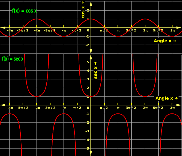
• The range in this case can be better understood if we analyze the graph of f(x) = cos x. It is shown in fig.3.29 below:

Fig.3.29

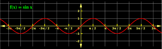
• The graph of f(x) = sin x, which we saw in the previous section, is given again below. This is for a comparison.

Fig.3.26

• An analysis of the cosine graph can be written in 3 steps:
(i) We already know the reason for the markings $\frac{\pi}{2},\; \pi,\; \frac{3\pi}{2},\; 2\pi,\; \frac{5\pi}{2}$ so on . . . on the x axis.
(ii) Now let us consider the output y values.
• We see that, whatever be the value of input x,
   ♦ Output y value (that is., cosine of x) never becomes greater than 1
   ♦ Output y value never becomes lesser than -1
(iii) We can mark any point on the red curve in the graph. The y coordinate of that point will be either 1 or -1 or a value between 1 and -1.
◼ So the range can be written as [-1, 1]
• That means:
   ♦ All real values between -1 and 1 are included in the range.
   ♦ Left side '[' indicates that -1 is also included in the range.
   ♦ Right side ']' indicates that +1 is also included in the range.

---

• We just saw that, cosine value can never rise above -1. Neither can it fall below -1.
• The reason can be written in 8 steps:
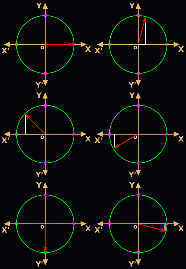
1. In the animation in fig.3.30 below, the thick white horizontal line is the base of the triangle in our familiar unit circle.

Fig.3.30

• We know that, this base is related to the cosine value of the angle.
2. The red ray starts to rotate from the +ve side of the x axis.
• Since the green circle is a unit circle, the length of the horizontal white line at this initial point will be 1
• As the rotation proceeds, the length of the horizontal line gradually decreases.
• It becomes zero when the ray completes a rotation of ${\frac{\pi}{2}}^c$. That is, when the ray coincides with the y axis.
• So we can write:
(i) The cosine value start to decrease from 1 (when the ray coincides with the +ve side of x axis)
(ii) The cosine value attains a value of 0 (when the ray coincides with the +ve side of y axis)
(iii) This decrease of cosine value, from 1 to zero, is indicated by the falling portion between x = 0 and x = $\frac{\pi}{2}$ in the graph in fig.3.29 above.
3. Next, the red ray proceeds to rotate from x = $\frac{\pi}{2}$ to x = π.
• We see that, the length of the horizontal white line increases from zero to 1.
• Though it is an 'increase in length', it happens on the negative side of the x axis. On this negative side, every x coordinate is negative, That means, on the negative side of the x axis, every cosine value is negative.
• As the length increases, the negative value increases. So in effect, it is a decrease.
• This decrease is indicated by the falling portion between x = $\frac{\pi}{2}$ and x = π in the graph in fig.3.29 above.
4. Next, the red ray proceeds to rotate from x = π to x = $\frac{3\pi}{2}$.
• We see that, the length of the horizontal white line decreases from 1 to zero.
• Though it is a 'decrease in length', it happens on the negative side of the x axis. On this negative side, every x values is negative, That means, on the negative side of the x axis, every cosine value is negative.
• As the length decreases, the negative value decreases. So in effect, it is an increase.
• This increase is indicated by the rising portion between x = π and x = $\frac{3\pi}{2}$ in the graph in fig.3.29 above.
5. Next, the red ray proceeds to rotate from x = $\frac{3\pi}{2}$ to x = 2π.
• We see that, the length of the horizontal white line increases from zero to 1.
• This increase is indicated by the rising portion between x = $\frac{3\pi}{2}$ and x = 2π in the graph in fig.3.29 above.
6. As the ray continues to rotate, this pattern repeats again and again. Thus we get the wave form on the positive side of the x axis in the graph.
7. Similar steps can be written for rotation in the anticlockwise direction also. Based on those steps, we will be able to explain the wave form on the negative side of the x axis in the graph.
8. Note that:
• In the first ${\frac{\pi}{2}}^c$ rotation in the anticlockwise direction, there is a fall in cosine value.
• In the first ${\frac{\pi}{2}}^c$ rotation in the clockwise direction also, there is a fall in cosine value.
• So there is a smooth transition between the two waves on either sides of the x axis.

---

Let us find the domain and range of f(x) = sec x. It can be written in 4 steps:
1. First we will find the domain:
• We have seen that:
    ♦ In the case of f(x) = sec x,
    ♦ $\frac{(2n+1)\pi}{2}$ where n is any integer, should not be used as input x
• So we can write:
Domain of f(x) = sec x is $R-\{x:x=\frac{(2n+1)\pi}{2},\; n\, \in \,Z\}$
• That means, we must subtract the set $\{x:x=\frac{(2n+1)\pi}{2},\; n\, \in \,Z\}$ from R. The resulting set after subtraction, is the domain of f(x) = sec x
• $\{x:x=\frac{(2n+1)\pi}{2},\; n\, \in \,Z\}$ is the set containing all $\frac{(2n+1)\pi}{2}$, where n is any integer.
2. Let us find the range of f(x) = sec x
• The range in this case can be better understood if we analyze the graph of f(x) = cos x and f(x) = sec x together. It is shown in fig.3.31 below:

Fig.3.31

An analysis of this graph can be written in 6 steps:
(i) Consider the segment from 0 to $\frac{\pi}{2}$ on the x axis.
• In this segment,
   ♦ the cosine curve falls
   ♦ but the secant curve rises.
• That means, when the angle increases from 0 to $\frac{\pi}{2}$,
   ♦ the cosine value decreases
   ♦ but the secant value increases.
• This is obvious because, secant is the reciprocal of cosine.
• In the segment from 0 to $\frac{\pi}{2}$, the maximum value of cosine occurs at zero
   ♦ So the minimum value of secant should also be at zero. 
   ♦ Indeed we see that, the rise of the secant curve occurs after zero.
• The value of cosine at zero is 1
   ♦ The value of secant at zero should be the reciprocal of 1, which is 1.
   ♦ Indeed we see that, the value of secant at zero is 1.
• The value of cosine at $\frac{\pi}{2}$ is 0
   ♦ The value of secant at $\frac{\pi}{2}$ should be the reciprocal of 0, which is not defined
   ♦ Indeed we see that, the value of secant curve never touches the vertical line through $\frac{\pi}{2}$
• As the angle approaches $\frac{\pi}{2}$, the cosine value becomes very small and consequently the secant which is the reciprocal, becomes very large.

◼ As seen before, we cannot put x = $\frac{\pi}{2}$ in $f(x) = \sec x = \frac{1}{\cos x}$. We can write: • As x approaches $\frac{\pi}{2}$, cos x becomes smaller and smaller, getting closer and closer to zero. (For example, values like 0.00001, 0.000001 are very close to zero) • As cos x becomes smaller and smaller, the reciprocal sec x becomes larger and larger. • This is indicated by the rising portion of the secant curve between 0 and $\frac{\pi}{2}$. • As angle becomes closer and closer to $\frac{\pi}{2}$, this rising portion gets closer and closer to the vertical line through $\frac{\pi}{2}$. (why does this happen? The reader may write the answer in his/her own notebooks) • But it never touches that vertical line. • If it touch, it would mean that, x = $\frac{\pi}{2}$ is a point in the secant curve. We know that, it cannot happen.

(ii) Consider the segment from $\frac{\pi}{2}$ to π on the x axis.
• In this segment,
   ♦ the cosine curve falls
   ♦ but the secant curve rises.
• That means, when the angle increases from $\frac{\pi}{2}$ to π,
   ♦ the cosine value decreases (increases negatively)
   ♦ but the secant value increases (decreases negatively).
• This is obvious because, secant is the reciprocal of cosine
Note that here, all the cosine values are -ve. Consequently, all the secant values will also be -ve.
• In the segment from $\frac{\pi}{2}$ to π, the minimum value of cosine occurs at π.
  ♦ So the maximum value of secant should also be at π.
  ♦ Indeed we see that, at π, the secant is at it's peak point in this segment.
  ♦ The value is reciprocal of -1, which is -1
(iii) Consider the segment from π to $\frac{3\pi}{2}$ on the x axis.
• In this segment,
   ♦ the cosine curve rises
   ♦ but the secant curve falls.
• That means, when the angle increases from π to $\frac{3\pi}{2}$,
   ♦ the cosine value increases
   ♦ but the secant value decreases.
• This is obvious because, secant is the reciprocal of cosine.
Note that here, all the cosine values are -ve. Consequently, all the secant values will also be -ve.
• In the segment from π to $\frac{3\pi}{2}$, the maximum value of cosine occurs at $\frac{3\pi}{2}$.
  ♦ So the minimum value of secant should also be at $\frac{3\pi}{2}$.
  ♦ Indeed we see that, as the angle approaches $\frac{3\pi}{2}$, the secant curve goes further and further down.

◼ As seen before, we cannot put x = $\frac{3\pi}{2}$ in $f(x) = \sec x = \frac{1}{\cos x}$. We can write: • As x approaches $\frac{3\pi}{2}$, cos x becomes smaller and smaller (negatively), getting closer and closer to zero. (For example, values like -0.00001, -0.000001 are very close to zero) • As cos x becomes smaller and smaller, the reciprocal sec x becomes larger and larger (negatively). • This is indicated by the falling portion of the secant curve between π and $\frac{3\pi}{2}$. • As angle becomes closer and closer to $\frac{3\pi}{2}$, this falling portion gets closer and closer to the vertical line through $\frac{3\pi}{2}$. (why does this happen? The reader may write the answer in his/her own notebooks) • But it never touches that vertical line. • If it touch, it would mean that, x = $\frac{3\pi}{2}$ is a point in the secant curve. We know that, it cannot happen.

(iv) Consider the segment from $\frac{3\pi}{2}$ to 2π on the x axis.
• In this segment,
   ♦ the cosine curve rises
   ♦ but the secant curve falls.
• That means, when the angle increases from $\frac{3\pi}{2}$ to 2π,
   ♦ the cosine value increases
   ♦ but the secant value decreases.
• This is obvious because, secant is the reciprocal of cosine.
Note that here, all the cosine values are +ve. Consequently, all the secant values will also be +ve.

(v) Now we have a basic idea about how the 'U' shapes and 'inverted U' shapes are formed in positive side of the x axis.
As the angle increases beyond 2π, this pattern repeats again and again.
(vi) Similar steps can be written for negative angles also. Those steps will explain the 'U' shapes and 'inverted U' shapes in the negative side of the x axis.
3. Based on the analysis of the graph, we can write:
• The output of f(x) = sec x can be any +ve real number starting from +1 and higher.
• The output of f(x) = sec x can be any -ve real number starting from -1 and lower.
• The values lying between -1 and +1 cannot be output values.
4. So the range of f(x) = sec is R - (-1, +1)
• That means, we have to subtract the set (-1, +1) from the the set of real numbers R
• The resulting set after subtraction is the range of f(x) = sec x
• (-1, +1) indicates that:
   ♦ all values between -1 and +1 are included in the set.
   ♦ '(' on the left side indicates that -1 is not included in the set.
   ♦ ')' on the right side indicates that +1 is not included in the set.
• So it is clear that, the two values -1 and +1 should not be subtracted from R.

---

In the next section, we will see domain and range of tangent and cotangent functions.

Previous

Contents

Next

Copyright©2021 Higher secondary mathematics.blogspot.com

Chapter 3.8 - Domain and Range of Sine and Cosecant Functions

In the previous section, we saw that any real number can be used as input x for f(x) = sin x and f(x) = cos x. So we get the feeling that, any real number can be used as input x for tan x, sec x etc., also. But it is not true. There are some exceptions. It can be written in 4 steps:

1. Consider f(x) = tan x.
• This can be written as $f(x)=\frac{\sin x}{\cos x}$
    ♦ So it is obvious that, cos x should not become zero.
• If we use an input x which makes cos x equal to zero, we will not get an output for the function f(x) = tan x.
• We know the exact x values for which cos x becomes zero. They are: $(2n+1)\frac{\pi}{2}$, where n is any integer.
◼ So we can write:
f(x) = tan x = $\frac{\sin x}{\cos x},\;x \neq (2n+1)\frac{\pi}{2}$ where n is any integer.
2. Consider f(x) = csc x.
• This can be written as $f(x)=\frac{1}{\sin x}$
    ♦ So it is obvious that, sin x should not become zero.
• If we use an input x which makes sin x equal to zero, we will not get an output for the function f(x) = csc x.
• We know the exact x values for which sin x becomes zero. They are: nπ, where n is any integer.
◼ So we can write:
f(x) = csc x = $\frac{1}{\sin x},\;x \neq n \pi$ where n is any integer.
3. Consider f(x) = sec x.
• This can be written as $f(x)=\frac{1}{\cos x}$
    ♦ So it is obvious that, cos x should not become zero.
• If we use an input x which makes cos x equal to zero, we will not get an output for the function f(x) = sec x.
• We know the exact x values for which cos x becomes zero. They are: $(2n+1)\frac{\pi}{2}$, where n is any integer.
◼ So we can write:
f(x) = sec x = $\frac{1}{\cos x},\;x \neq (2n+1)\frac{\pi}{2}$ where n is any integer.
4. Consider f(x) = cot x.
• This can be written as $f(x)=\frac{\cos x}{\sin x}$
    ♦ So it is obvious that, sin x should not become zero.
• If we use an input x which makes sin x equal to zero, we will not get an output for the function f(x) = cot x.
• We know the exact x values for which sin x becomes zero. They are: nπ, where n is any integer.
◼ So we can write:
f(x) = cot x = $\frac{\cos x}{\sin x},\;x \neq n \pi$ where n is any integer.

---

Sign of trigonometric functions

This can be written in 4 steps:
1. Consider the unit circle that we saw in the previous sections. In that circle, we have three important items:
(i) The tip of the ray.
   ♦ We denoted it as P.
(ii) Base of the triangle OMP.
   ♦ We denoted it as a
(iii) Altitude of the triangle OMP.
   ♦ We denoted it as b
2. We know that:
Coordinates of P are written using a and b.
3. We also know that:
  ♦ a is related to cosine
  ♦ b is related to sine
4. Based on steps (1), (2) and (3), we can write about the four quadrants:
First quadrant
(i) If P is in the I quadrant, the coordinates of P will be (a, b)
(ii) We know that:
   ♦ x coordinate is the cosine.
   ♦ y coordinate is the sine.
(iii) So in the I quadrant, cosine will be +ve, sine will be +ve.
• Consequently,
sec will be +ve, csc will be +ve.
• Also,
tan will be +ve, cot will be +ve
(iv) Thus we get the column named I in the table 3.1 below:

Table 3.1

• Note that, the ray can rotate in the anticlockwise direction (to give a positive angle) and reach the I quadrant.
• The ray can also rotate in the clockwise direction (to give a negative angle) and reach the I quadrant.
• What ever be the direction of rotation, the coordinates of P will not change. So the signs written in the column named I of table 3.1 is valid for both +ve and -ve angles.

Second quadrant
(i) If P is in the II quadrant, the coordinates of P will be (-a, b)
(ii) We know that:
   ♦ x coordinate is the cosine.
   ♦ y coordinate is the sine.
(iii) So in the II quadrant, cosine will be -ve, sine will be +ve.
• Consequently,
sec will be -ve, csc will be +ve.
• Also,
tan will be -ve, cot will be -ve
(iv) Thus we get the column named II in the table 3.1 above.
• Note that, the ray can rotate in the anticlockwise direction (to give a positive angle) and reach the II quadrant.
• The ray can also rotate in the clockwise direction (to give a negative angle) and reach the II quadrant.
• What ever be the direction of rotation, the coordinates of P will not change. So the signs written in the column named II of table 3.1 is valid for both +ve and -ve angles. 

Third quadrant
(i) If P is in the III quadrant, the coordinates of P will be (-a, -b)
(ii) We know that:
   ♦ x coordinate is the cosine.
   ♦ y coordinate is the sine.
(iii) So in the III quadrant, cosine will be -ve, sine will be -ve.
• Consequently,
sec will be -ve, csc will be -ve.
• Also,
tan will be +ve, cot will be +ve
(iv) Thus we get the column named III in the table 3.1 above.
• Note that, the ray can rotate in the anticlockwise direction (to give a positive angle) and reach the III quadrant.
• The ray can also rotate in the clockwise direction (to give a negative angle) and reach the III quadrant.
• What ever be the direction of rotation, the coordinates of P will not change. So the signs written in the column named III of table 3.1 are valid for both +ve and -ve angles. 

Fourth quadrant
(i) If P is in the IV quadrant, the coordinates of P will be (a, -b)
(ii) We know that:
   ♦ x coordinate is the cosine.
   ♦ y coordinate is the sine.
(iii) So in the IV quadrant, cosine will be +ve, sine will be -ve.
• Consequently,
sec will be +ve, csc will be -ve.
• Also,
tan will be -ve, cot will be -ve
(iv) Thus we get the column named IV in the table 3.1 above.
• Note that, the ray can rotate in the anticlockwise direction (to give a positive angle) and reach the IV quadrant.
• The ray can also rotate in the clockwise direction (to give a negative angle) and reach the IV quadrant.
• What ever be the direction of rotation, the coordinates of P will not change. So the signs written in the column named IV of table 3.1 are valid for both +ve and -ve angles.

---

Domain and range of trigonometric functions

This can be explained in 2 steps:
1. We know that:
• Domain of a function is the set containing all the input x values.
• Range of a function is the set containing all the output y [y is same as f(x)] values.
2. We need to have a basic idea about the domain and range of the various trigonometric functions like f(x) = sin x, f(x) = cos x, f(x) = sec x etc.,

---

Let us find the domain and range of f(x) = sin x. It can be written in 2 steps:
1. First we will find the domain:
• We have seen that:
In the case of f(x) =sin x, any real number can be used as input x.
• So we can write: Domain of f(x) = sin x, is the set R.
(Recall that, R is the set of real numbers)
2. Let us find the range of f(x) = sin x
The range in this case can be better understood if we analyze the graph of f(x) = sin x. It is shown in fig.3.26 below:

Fig.3.26

• An analysis of this graph can be written in 4 steps:
(i) We see that, on the x axis, the markings are: $\frac{\pi}{2},\; \pi,\; \frac{3\pi}{2},\; 2\pi,\; \frac{5\pi}{2}$ so on . . .
• Normally, we expect markings as: 1, 2, 3, . . . OR  5, 10, 15, . . .
• The markings in the above graph are no different from 1, 2, 3, . . . OR  5, 10, 15, .
• If we use the real number line as the x axis, this type of marking can be achieved by putting marks at $\frac{3.14}{2},\; 3.14,\; \frac{3\times 3.14}{2},\; 2\times 3.14,\; \frac{5\times 3.14}{2}$ so on . . .
• Here each unit on the x axis is ${\frac{\pi}{2}}^c$
• These markings can go up to +∞. That means, all positive real numbers can be used as input x.
• They are positive angles obtained when the ray rotates in the anticlockwise direction.
(ii) Similar is the case with markings on the negative side of the x axis.
• They are negative angles, which are obtained when the ray rotates in the clockwise direction.
• The -ve markings can go up to -∞. That means, all negative real numbers can be used as input x.
(iii) Now let us consider the output y values.
• We see that, whatever be the value of input x,
   ♦ Output y value (that is., sine of x) never becomes greater than 1
   ♦ Output y value never becomes lesser than -1
(iv) We can mark any point on the red curve in the graph. The y coordinate of that point will be either 1 or -1 or a value between 1 and -1.
◼ So the range can be written as [-1, 1]
• That means:
   ♦ All real values between -1 and 1 are included in the range.
   ♦ Left side '[' indicates that -1 is also included in the range.
   ♦ Right side ']' indicates that +1 is also included in the range.

---

• We just saw that sine value can never rise above +1. Neither can it fall below -1.
• The reason can be written in 8 steps:
1. In the animation in fig.3.27 below, the thick white vertical line is the altitude of the triangle in our familiar unit circle.

Fig.3.27

• We know that, this altitude is related to the sine value of the angle.
2. The red ray starts to rotate from the +ve side of the x axis.
• As the rotation proceeds, the length of the white vertical line gradually increases.
• It becomes maximum when the ray completes a rotation of ${\frac{\pi}{2}}^c$. That is, when the ray coincides with the y axis.
• Since the green circle is a unit circle, the length of the vertical white line at this point will be 1
• So we can write:
(i) The sine value start to increase from zero (when the ray coincides with the +ve side of x axis)
(ii) The sine value attains a maximum value of 1 (when the ray coincides with the +ve side of y axis)
(iii) This increase of sine value, from zero to 1, is indicated by the rising portion between x = 0 and x = $\frac{\pi}{2}$ in the graph in fig.3.26 above.
3. Next, the red ray proceeds to rotate from x = $\frac{\pi}{2}$ to x = π.
• We see that, the length of the vertical white line decreases from 1 to zero.
• This decrease is indicated by the falling portion between x = $\frac{\pi}{2}$ and x = π in the graph in fig.3.26 above.
4. Next, the red ray proceeds to rotate from x = π to x = $\frac{3\pi}{2}$.
• We see that, the length of the vertical white line increases from zero to 1.
• Though it is an 'increase in length', it happens below the x axis. Below the x axis, every y coordinate is negative. That means, below the y axis, every sine value is negative.
• As the length increases, the negative value increases. So in effect, it is a decrease.
• This decrease is indicated by the falling portion between x = π and x = $\frac{3\pi}{2}$ in the graph in fig.3.26 above.
5. Next, the red ray proceeds to rotate from x = $\frac{3\pi}{2}$ to x = 2π.
• We see that, the length of the vertical white line decreases from 1 to zero.
• Though it is a 'decrease in length', it happens below the x axis. Below the x axis, every y coordinate is negative, That means, below the y axis, every sine value is negative.
• As the length decreases, the negative value decreases. So in effect, it is an increase.
• This increase is indicated by the rising portion between x = $\frac{3\pi}{2}$ and x = 2π in the graph in fig.3.26 above.
6. As the ray continues to rotate, this pattern repeats again and again. Thus we get the wave form on the positive side of the x axis in the graph.
7. Similar steps can be written for rotation in the anticlockwise direction also. Based on those steps, we will be able to explain the wave form on the negative side of the x axis in the graph.
8. Note that:
• In the first ${\frac{\pi}{2}}^c$ rotation in the anticlockwise direction, there is a rise in sine value.
• In the first ${\frac{\pi}{2}}^c$ rotation in the clockwise direction, there is a fall in sine value.
• So there is a smooth transition between the two waves on either sides of the x axis.

---

Let us find the domain and range of f(x) = csc x. It can be written in 4 steps:
1. First we will find the domain:
• We have seen that:
    ♦ In the case of f(x) = csc x,
    ♦ nπ where n is any integer, should not be used as input x
• So we can write:
Domain of f(x) = csc x is R -{x : x = nπ, n ∈ Z}
• That means, we must subtract {x : x = nπ, n ∈ Z} from R. The resulting set after subtraction, is the domain of f(x) = csc x
• {x : x = nπ, n ∈ Z} is the set containing all nπ, where n is any integer.
2. Let us find the range of f(x) = csc x
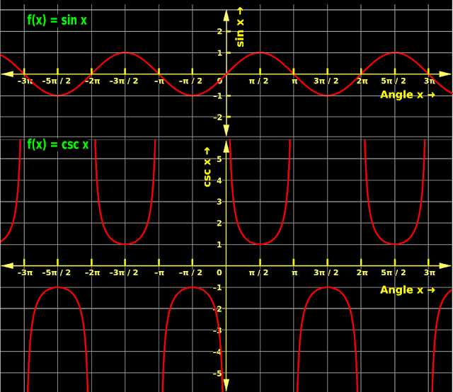
We know that, csc is the reciprocal of sine. So the range of f(x) = csc x can be better understood if we analyze the graph of f(x) = sin x and f(x) = csc x together. It is shown in fig.3.28 below:

Fig.3.28

An analysis of this graph can be written in 6 steps:
(i) Consider the segment from 0 to $\frac{\pi}{2}$ on the x axis.
• In this segment,
   ♦ the sine curve rises
   ♦ but the csc curve falls.
• That means, when the angle increases from 0 to $\frac{\pi}{2}$,
   ♦ the sine value increases
   ♦ but the csc value decreases.
• This is obvious because, csc is the reciprocal of sine
• In the segment from 0 to $\frac{\pi}{2}$, the maximum value of sine occurs at $\frac{\pi}{2}$
   ♦ So the minimum value of csc should also be at $\frac{\pi}{2}$   
   ♦ Indeed we see that, the fall of the csc curve occurs upto $\frac{\pi}{2}$.
   ♦ Thereafter, it rises.
• The value of sine at $\frac{\pi}{2}$ is 1
   ♦ The value of csc at $\frac{\pi}{2}$ should be the reciprocal of 1, which is 1
   ♦ Indeed we see that, the value of csc at $\frac{\pi}{2}$ is 1
(ii) Consider the segment from $\frac{\pi}{2}$ to π on the x axis.
• In this segment,
   ♦ the sine curve falls
   ♦ but the csc curve rises.
• That means, when the angle increases from $\frac{\pi}{2}$ to π,
   ♦ the sine value decreases
   ♦ but the csc value increases.
• This is obvious because, csc is the reciprocal of sine
• In the segment from $\frac{\pi}{2}$ to π, the minimum value of sine occurs at π.
  ♦ So the maximum value of csc should also be at π.
  ♦ Indeed we see that, as π approaches, the csc curve rises further and further up.

◼ As seen before, we cannot put x = π in $f(x) = \csc x = \frac{1}{\sin x}$. We can write: • As x approaches π, sin x becomes smaller and smaller, getting closer and closer to zero. (For example, values like 0.00001, 0.000001 are very close to zero) • As sin x becomes smaller and smaller, the reciprocal csc x becomes larger and larger. • This is indicated by the rising portion of the csc curve between $\frac{\pi}{2}$ and π. • As angle becomes closer and closer to π, this rising portion gets closer and closer to the vertical line through π. (why does this happen? The reader may write the answer in his/her own notebooks) • But it never touches that vertical line. • If it touch, it would mean that, x = π is a point in the csc curve. We know that, it cannot happen.

(iii) Consider the segment from π to $\frac{3\pi}{2}$ on the x axis.
• In this segment,
   ♦ the sine curve falls
   ♦ but the csc curve rises.
• That means, when the angle increases from π to $\frac{3\pi}{2}$,
   ♦ the sine value decreases
   ♦ but the csc value increases.
• This is obvious because, csc is the reciprocal of sine.
Note that here, all the sine values are -ve. Consequently, all the csc values will also be -ve.
• In the segment from π to $\frac{3\pi}{2}$, the minimum value of sine occurs at $\frac{3\pi}{2}$.
  ♦ So the maximum value of csc should also be at $\frac{3\pi}{2}$.
   ♦ Indeed we see that, the rise of the csc curve occurs upto $\frac{3\pi}{2}$.
   ♦ Thereafter, it falls.
• The value of sine at $\frac{3\pi}{2}$ is -1
   ♦ The value of csc at $\frac{3\pi}{2}$ should be the reciprocal of -1, which is -1.
   ♦ Indeed we see that, the value of csc at $\frac{3\pi}{2}$ is -1.
• Consider the portion just after π. The sine values here will be very small negative values. Consequently, the csc values here will be very large negative values. This fact can be clearly seen in the graphs.
(iv) Consider the segment from $\frac{3\pi}{2}$ to 2π on the x axis.
• In this segment,
   ♦ the sine curve rises
   ♦ but the csc curve falls.
• That means, when the angle increases from $\frac{3\pi}{2}$ to 2π,
   ♦ the sine value increases
   ♦ but the csc value decreases.
• This is obvious because, csc is the reciprocal of sine.
Note that here, all the sine values are -ve. Consequently, all the csc values will also be -ve.

◼ As seen before, we cannot put x = 2π in $f(x) = \csc x = \frac{1}{\sin x}$. We can write: • As x approaches 2π, sin x becomes smaller and smaller (negatively), getting closer and closer to zero. (For example, values like -0.00001, -0.000001 are very close to zero) • As sin x becomes smaller and smaller (negatively), the reciprocal csc x becomes larger and larger (negatively). • This is indicated by the falling portion of the csc curve between $\frac{3\pi}{2}$ and 2π. • As angle becomes closer and closer to 2π, this falling portion gets closer and closer to the vertical line through 2π. (why does this happen? The reader may write the answer in his/her own notebooks) • But it never touches that vertical line. • If it touch, it would mean that, x = 2π is a point in the csc curve. We know that, it cannot happen.

(v) Now we have a basic idea about how the 'U' shapes and 'inverted U' shapes are formed in positive side of the x axis.
• As the angle increases beyond 2π, this pattern repeats again and again.
(vi) Similar steps can be written for negative angles also. Those steps will explain the 'U' shapes and 'inverted U' shapes in the negative side of the x axis.
3. Based on the analysis of the graph, we can write:
• The output of f(x) = csc x can be any +ve real number starting from +1 and higher.
• The output of f(x) = csc x can be any -ve real number starting from -1 and lower.
• The values lying between -1 and +1 cannot be outpit values.
4. So the range of f(x) = csc is R - (-1, +1)
• That means, we have to subtract the set (-1, +1) from the the set of real numbers R
• The resulting set after subtraction is the range of f(x) = csc x
• (-1, +1) indicates that:
   ♦ all values between -1 and +1 are inculded in the set (-1, +1).
   ♦ '(' on the left side indicates that -1 is not included in the set (-1, +1).
   ♦ ')' on the right side indicates that +1 is not included in the set (-1, +1).
• So it is clear that, the two values -1 and +1 should not be subtracted from R.

---

In the next section, we will see domain and range of cosine and secant functions.

Previous

Contents

Next

Copyright©2021 Higher secondary mathematics.blogspot.com