Showing posts with label second order derivatives. Show all posts

Wednesday, January 1, 2025

22.22 - Miscellaneous Examples on Applications of Derivatives - Part 4

In the previous section, we saw some miscellaneous examples. In this section, we will see a few more miscellaneous examples.

Solved example 22.82
A circular disc of radius 3 cm is being heated. Due to expansion, it's radius increases at the rate of 0.05 cm/s. Find the rate at which its area is increasing when radius is 3.2 cm.
Solution:
1. We have the formula for area of a circle: A = πr2.
2. The radius increases at the rate of 0.05 cm/s.
• So radius at time t will be 0.05t
4. So area A at time t = π(0.05t)2 = 0.0025πt2 cm2
• Now the rate of change of area w.r.t radius can be obtained as:
dA/dt = 0.0025π(2t) = 0.005 πt cm2/s
• This result can be used to find the rate of change of area at any instant.
5. We want the rate when radius is 3.2 cm. So we want the instant at which the radius is 3.2 cm. For that, we can use the result in (2). We get:
3.2 = 0.05t
⇒ t = 64
6. So from (4) we get:
(dA/dt)t=64 = 0.005π(64) = 0.320π cm2/s

Solved example 22.83
An open topped box is to be constructed by removing equal squares from each corner of a 3 metre by 8 metre rectangular sheet of aluminium and folding up the sides. Find the volume of the largest such box.
Solution:
Step I: Writing the problem as a function
1. In fig.22.77 below, the original rectangular sheet is shown in yellow color. Red squares are cut off from the corners.

Fig.22.77

• So when the flaps are folded up, we will get a box with:
   ♦ base a rectangle (8 − 2x) × (3 − 2x) m2
   ♦ height x m
• Then the volume of the box = x(8 − 2x)(3 − 2x) m3

2. It is clear that, V depends on x. That means, V is a function of x. So we can write:
V = f(x) = x(8 − 2x)(3 − 2x) m3

3. We want V to be as large as possible. That means, we want the largest of all local maxima of f. That means, we need to find all local maxima and compare them.

Step II: Finding the critical points
1. Write the first two derivatives:
f '(x) =12x2 − 44x + 24

f ''(x) = 24x − 44

2. Equate the first derivative to zero and solve for x:
12x2 − 44x + 24 = 0
⇒ x = 2/3, x = 3 

3. So the only two points in category I are: x = 2/3 and x = 3
4. We obtained f '(x) = 12x2 − 44x + 24
• This function is defined for all real numbers. That means, there is no input x at which f '(x) is not defined.
• Therefore, there will be no points in category II.
5. So the only two critical points are: x = 2/3 and x = 3

Step III: Find f ''(x) at the critical points
1. f ''(2/3) = 24(2/3) − 44 = −28
2. f ''(3) =  24(3) − 44 = 28

Step IV: Applying the second derivative test
1. Since f ''(2/3) is −ve, there is a local maximum at x = 2/3
2. Since f ''(3) is +ve, there is a local minimum at x = 3

Step V: Finding the actual maximum value:
• The local maximum value at x = 2/3 is given by:
f(2/3) = (2/3)[8 − 2(2/3)][3 − 2(2/3)] = 200/27 m3.

Solved example 22.84
Manufacturer can sell x items at a price of rupees $\rm{5 - \frac{x}{100}}$ each. The cost price of x items is Rs $\rm{\frac{x}{5} + 500}$. Find the number of items he should sell to earn maximum profit.
Solution:
Step I: Writing the problem as a function
1. When the manufacturer sells x items, he will get an income of: Rs $\rm{x\left(5 - \frac{x}{100} \right)}$
2. To produce those x items, he would have spent:
Rs $\rm{\frac{x}{5} + 500}$
3. So the profit P can be obtained as:
$\rm{P\,=\, x\left(5 - \frac{x}{100} \right)~-~\frac{x}{5} + 500}$
4. It is clear that, P depends on x. That means, P is a function of x. So we can write:
$\rm{P\,=\, f(x)\,=\,x\left(5 - \frac{x}{100} \right)~-~\frac{x}{5} + 500}$
5. We want P to be as large as possible. That means, we want the largest of all local maxima of f. That means, we need to find all local maxima and compare them.

Step II: Finding the critical points
1. Write the first two derivatives:
f '(x) = $\rm{\frac{-x}{50} + \frac{24}{5}}$

f ''(x) = $\rm{\frac{-1}{50}}$

2. Equate the first derivative to zero and solve for x:
$\rm{\frac{-x}{50} + \frac{25}{4} \,=\, 0}$
⇒ x = 240

3. So the only one point in category I is: x = 240
4. We obtained f '(x) = $\rm{\frac{-x}{50} + \frac{24}{5}}$
• This function is defined for all real numbers. That means, there is no input x at which f '(x) is not defined.
• Therefore, there will be no points in category II.
5. So the only one critical point is: x = 240

Step III: Find f ''(x) at the critical points
f ''(x) is a constant: $\rm{\frac{-1}{50}}$

Step IV: Applying the second derivative test
• Since f ''(240) is −ve, there is a local maximum at x = 240

Step V: Final result:
• For maximum profit, the manufacturer must sell 240 items.

Solved example 22.85
Find the maximum area of an isosceles triangle inscribed in the ellipse $\rm{\frac{x^2}{a^2}\,+\,\frac{y^2}{b^2}\,=\,1}$ with it's vertex at one end of the major axis.
Solution:
Step I: Writing the problem as a function
1. The given ellipse is: $\rm{\frac{x^2}{a^2}\,+\,\frac{y^2}{b^2}\,=\,1}$
• So it is clear that:
    ♦ Major axis lies along the x-axis.
    ♦ Minor axis lies along the y-axis.
    ♦ Center of ellipse is at the origin O.
2. Thus we get fig.22.78 below:

Fig.22.78

• The vertex A of the isosceles triangle is at one end of the major axis.
3. Let the base of the isosceles triangle intersect the x-axis at D(h,0).
• Then the y-coordinates of B and C can be obtained as shown below:

$\begin{array}{ll} {~\color{magenta}    1    }    &{{}}    &{\frac{x^2}{a^2}\,+\,\frac{y^2}{b^2}}    & {~=~}    &{1}    \\
{~\color{magenta}    2    }    &{\implies}    &{\frac{h^2}{a^2}\,+\,\frac{y^2}{b^2}}    & {~=~}    &{1}    \\
{~\color{magenta}    3    }    &{\implies}    &{\frac{y^2}{b^2}}    & {~=~}    &{1~-~\frac{h^2}{a^2}}    \\
{~\color{magenta}    4    }    &{\implies}    &{y^2}    & {~=~}    &{b^2 \left(1~-~\frac{h^2}{a^2} \right)}    \\
{~\color{magenta}    5    }    &{\implies}    &{y}    & {~=~}    &{\pm \sqrt{b^2 \left(1~-~\frac{h^2}{a^2} \right)}}    \\
\end{array}$

• So the y-coordinate of B is $\sqrt{b^2 \left(1~-~\frac{h^2}{a^2} \right)}$
• And the y-coordinate of C is $-\sqrt{b^2 \left(1~-~\frac{h^2}{a^2} \right)}$
• Then the distance BC will be $2 \sqrt{b^2 \left(1~-~\frac{h^2}{a^2} \right)}$
4. Next we want the coordinates of A. It can be calculated as shown below:

$\begin{array}{ll} {~\color{magenta}    1    }    &{{}}    &{\frac{x^2}{a^2}\,+\,\frac{y^2}{b^2}}    & {~=~}    &{1}    \\
{~\color{magenta}    2    }    &{\implies}    &{\frac{x^2}{a^2}\,+\,\frac{0^2}{b^2}}    & {~=~}    &{1}    \\
{~\color{magenta}    3    }    &{\implies}    &{\frac{x^2}{a^2}}    & {~=~}    &{1}    \\
{~\color{magenta}    4    }    &{\implies}    &{x^2}    & {~=~}    &{a^2}    \\
{~\color{magenta}    5    }    &{\implies}    &{x}    & {~=~}    &{\pm a}    \\
\end{array}$

• So the coordinates of A are: (a,0).
• Then the altitude AD = (h+a)
5. Now we can write the expression for the area of triangle ABC:
Area = 1/2 × Base × Altitude = 1/2 × BC × AD
= $\frac{1}{2} × 2 \sqrt{b^2 \left(1~-~\frac{h^2}{a^2} \right)} × (h+a)$
• This can be simplified as:

$\begin{array}{ll} {~\color{magenta}    1    }    &{{}}    &{\text{Area}}    & {~=~}    &{\frac{1}{2} × 2 \sqrt{b^2 \left(1~-~\frac{h^2}{a^2} \right)} × (h+a)}    \\
{~\color{magenta}    2    }    &{{}}    &{{}}    & {~=~}    &{b \sqrt{\left(1~-~\frac{h^2}{a^2} \right)} × (h+a)}    \\
{~\color{magenta}    3    }    &{{}}    &{{}}    & {~=~}    &{b \sqrt{\left(\frac{a^2 – h^2}{a^2} \right)} × (h+a)}    \\
{~\color{magenta}    4    }    &{{}}    &{{}}    & {~=~}    &{\frac{b}{a} \sqrt{\left(a^2 – h^2 \right)} × (h+a)}    \\
\end{array}$

6. It is clear that, Area A depends on h. That means, A is a function of h. So we can write:
$\rm{A\,=\, f(x)\,=\,\frac{b}{a} \sqrt{\left(a^2 – h^2 \right)} × (h+a)}$
5. We want A to be as large as possible. That means, we want the largest of all local maxima of f. That means, we need to find all local maxima and compare them.

Step II: Finding the critical points
1. Write the first two derivatives:

$\begin{array}{ll} {~\color{magenta}    1    }    &{{}}    &{f(h)}    & {~=~}    &{\frac{b}{a} \sqrt{\left(a^2 – h^2 \right)} × (h+a)}    \\
{~\color{magenta}    2    }    &{\implies}    &{f'(h)}    & {~=~}    &{\frac{b}{a} \left[\sqrt{\left(a^2 – h^2 \right)} × (1) ~+~(h+a) (1/2) \left(a^2 – h^2 \right)^{-1/2} (-2h) \right]}    \\
{~\color{magenta}    3    }    &{{}}    &{{}}    & {~=~}    &{\frac{b}{a} \left[\sqrt{\left(a^2 – h^2 \right)}  ~-~ \frac{h(h+a)}{\sqrt{\left(a^2 – h^2 \right)}} \right]}    \\
{~\color{magenta}    4    }    &{{}}    &{{}}    & {~=~}    &{\frac{b}{a} \left[\frac{a^2 – h^2 ~-~h(h+a)}{\sqrt{\left(a^2 – h^2 \right)}} \right]}    \\
{~\color{magenta}    5    }    &{{}}    &{{}}    & {~=~}    &{\frac{b}{a} \left[\frac{a^2 – h^2 – h^2 – ha}{\sqrt{\left(a^2 – h^2 \right)}} \right]}    \\
{~\color{magenta}    6    }    &{{}}    &{{}}    & {~=~}    &{\frac{b}{a} \left[\frac{a^2 – 2 h^2  – ha}{\sqrt{\left(a^2 – h^2 \right)}} \right]}    \\
\end{array}$                           

• In this problem, calculation of f ''(h) will be a lengthy process. So we will use the first derivative test

2. Equate the first derivative to zero and solve for h:
$\rm{a^2 – 2 h^2  – ha \,=\, 0}$
⇒ $\rm{2 h^2 + ha - a^2 \,=\, 0}$
• Using quadratic formula, we get:
h = a/2 and h = −a
• h cannot be −a. Because, then in fig.22.78 above, D will coincide with the left end of the major axis. Parts of the triangle will fall outside the ellipse.

3. So the only one point in category I is: x = a/2
4. We obtained f '(h) = $\frac{b}{a} \left[\frac{a^2 – 2 h^2  – ha}{\sqrt{\left(a^2 – h^2 \right)}} \right]$
• This function is not defined when h = a. But when h = a, the function itself becomes invalid because there will be no inscribed triangle.
• Therefore, there will be no points in category II.
5. So the only one critical point is: h = a/2
6. The domain is (−a,a).
• Based on the critical point, the domain can be divided into two intervals: (−a, a/2) and (a/2, a)

Step III: Analyzing the signs of f '(x) in the two intervals
1. Consider the first interval. Zero is a convenient point.
• We get:
$\begin{array}{ll} {~\color{magenta}    1    }    &{{}}    &{f'(h)}    & {~=~}    &{\frac{b}{a} \left[\frac{a^2 – 2 h^2  – ha}{\sqrt{\left(a^2 – h^2 \right)}} \right]}    \\
{~\color{magenta}    2    }    &{\implies}    &{f'(0)}    & {~=~}    &{\frac{b}{a} \left[\frac{a^2 – 2 (0)^2  – (0)a}{\sqrt{\left(a^2 – (0)^2 \right)}} \right]}    \\
{~\color{magenta}    3    }    &{{}}    &{{}}    & {~=~}    &{\frac{b}{a} \left[\frac{a^2}{\sqrt{\left(a^2 \right)}} \right]}    \\
{~\color{magenta}    4    }    &{{}}    &{{}}    & {~=~}    &{b}    \\
\end{array}$

• So in the first interval. f '(x) is +ve.

2. Consider the second interval. $\frac{3a}{4}$  is a convenient point.
• We get:
$\begin{array}{ll} {~\color{magenta}    1    }    &{{}}    &{f'(h)}    & {~=~}    &{\frac{b}{a} \left[\frac{a^2 – 2 h^2  – ha}{\sqrt{\left(a^2 – h^2 \right)}} \right]}    \\
{~\color{magenta}    2    }    &{\implies}    &{f'(3a/4)}    & {~=~}    &{\frac{b}{a} \left[\frac{a^2 – 2 (3a/4)^2  – (3a/4)a}{\sqrt{\left(a^2 – (3a/4)^2 \right)}} \right]}    \\
{~\color{magenta}    3    }    &{{}}    &{{}}    & {~=~}    &{\frac{b}{a} \left[\frac{a^2 – 2 \left(\frac{9 a^2}{16} \right)  – \frac{3 a^2}{4}}{\sqrt{\left(a^2 – \frac{9 a^2}{16} \right)}} \right]}    \\
{~\color{magenta}    4    }    &{{}}    &{{}}    & {~=~}    &{\frac{b}{a} \left[\frac{\frac{16 a^2 - 18 a^2 – 12 a^2}{16}}{\sqrt{\left(\frac{16 a^2 – 9 a^2}{16} \right)}} \right]}    \\
{~\color{magenta}    5    }    &{{}}    &{{}}    & {~=~}    &{\frac{b}{a} \left[\frac{\frac{16 a^2 - 30 a^2}{16}}{\sqrt{\left(\frac{7 a^2}{16} \right)}} \right]}    \\
{~\color{magenta}    6    }    &{{}}    &{{}}    & {~=~}    &{\frac{b}{a} \left[\frac{\frac{- 14 a^2}{16}}{\sqrt{\left(\frac{7 a^2}{16} \right)}} \right]}    \\
\end{array}$

• So in the second interval. f '(x) is −ve.

Step IV: Applying the first derivative test
• Since f '(x) changes sign from +ve to −ve at the critical point, we have a maximum at that critical point.

Step V: Final result:
• For maximum area, h = a/2
So from step I, we get:

$\begin{array}{ll} {~\color{magenta}    1    }    &{{}}    &{\text{Area}}    & {~=~}    &{\frac{1}{2} × 2 \sqrt{b^2 \left(1~-~\frac{h^2}{a^2} \right)} × (h+a)}    \\
{~\color{magenta}    2    }    &{\implies}    &{\text{Area (max)}}    & {~=~}    &{\sqrt{b^2 \left(1~-~\frac{(a/2)^2}{a^2} \right)} × ((a/2)+a)}    \\
{~\color{magenta}    3    }    &{{}}    &{{}}    & {~=~}    &{\sqrt{b^2 \left(1~-~\frac{a^2 / 4}{a^2} \right)} × (3a/2)}    \\
{~\color{magenta}    4    }    &{{}}    &{{}}    & {~=~}    &{\sqrt{3 b^2 / 4} × (3a/2)}    \\
{~\color{magenta}    5    }    &{{}}    &{{}}    & {~=~}    &{\frac{\sqrt{3} b}{2} × \frac{3a}{2}}    \\
{~\color{magenta}    6    }    &{{}}    &{{}}    & {~=~}    &{\frac{3 \sqrt{3} \,ab}{4}}    \\
\end{array}$


The link below gives a few more miscellaneous examples:

Miscellaneous Exercise


We have completed this chapter on applications of derivatives. In the next chapter, we will see Integrals.

Previous

Contents

Next

Copyright©2024 Higher secondary mathematics.blogspot.com

Sunday, November 17, 2024

22.17 - The Second Derivative Test

In the previous section, we saw the concavity test. In this section, we will see the second derivative test for finding local extrema.

1. Consider the graph in fig.22.55 of the previous section. With some modifications, it is shown again below as fig.22.57.
• Two modifications are made to the earlier fig.22.55
(i) The point (0,0) is specially marked because, it is a local maximum.
(ii) The vertical white dashed line is drawn through the local minimum. This is for getting a better understanding about the change of sign of f ' on either sides of the local minimum. Such a line should have to be drawn through the local maximum also. But there, we already have the y-axis.

Fig.22.57

• The vertical magenta dashed line divides the graph into two portions: concave down portion and concave up portion.

2. Consider the concave down portion. Any concave down portion will contain a peak point. This peak point will be a local maximum. We want a relation between this local maximum and the second derivative f ''. The relation can be established in 4 steps:
(i) We see that, in the concave down portion:
   ♦ The green line is below the x-axis.
   ♦ This happens because, in this portion, all f '' values are −ve. We have seen the reason in the previous section 22.16.
(ii) We see that, in the concave down portion:
• The yellow curve is above x-axis up to the local maximum.
   ♦ This happens because, in this portion, all f ' values are +ve upto the local maximum. We have seen the reason in a previous section. See fig.22.46(b) of section 22.15.
• The yellow curve is below x-axis after the local maximum.
   ♦ This happens because, in this portion, all f ' values are −ve after the local maximum. We have seen the reason in a previous section. See fig.22.46(b) of section 22.15.
(iii) We see that, in the concave down portion:
• The yellow curve changes sign at the local maximum. That means, f ' changes sign at the local maximum.
(We know that, at the point where the "change in sign" occurs, f ' will be zero)
(iv) Based on the above three steps, we can establish the relation:
• At the local maximum:
   ♦ f ' will be zero.
   ♦ f '' will be −ve.

3. Consider the concave up region. Any concave up region will contain a valley point. This valley point will be a local minimum . We want a relation between this local minimum and the second derivative f ''. The relation can be established in 4 steps:
(i) We see that, in the concave up portion:
   ♦ The green line is above the x-axis.
   ♦ This is because, in this portion, all f '' values are +ve. We have seen the reason in the previous section 22.16.
(ii) We see that, in the concave up portion:
• The yellow curve is below x-axis up to the local minimum.
   ♦ This happens because, in this portion, all f ' values are −ve up to the local minimum. We have seen the reason in a previous section. See fig.22.46(a) of section 22.15.
• The yellow curve is above x-axis after the local maximum.
   ♦ This happens because, in this portion, all f ' values are +ve after the local maximum. We have seen the reason in a previous section. See fig.22.46(a) of section 22.15.
(iii) We see that, in the concave up portion:
• The yellow curve changes sign at the local minimum. That means, f ' changes sign at the local minimum.
(We know that, at the point where the "change in sign" occurs, f ' will be zero)
(iv) Based on the above three steps, we can establish the relation:
• At the local minimum:
   ♦ f ' will be zero.
   ♦ f '' will be +ve.
4. So now we have an effective test to determine whether a critical point is a local maximum or a local minimum. The test can be done in 2 steps:
Step I: Determine all critical points
Step II: Determine the sign of f '' at each of those points.
   ♦ If f '' is −ve at a critical point, then that point is a local maximum.
   ♦ If f '' is +ve at a critical point, then that point is a local minimum.
◼ This test is known as the second derivative test.


• Note that, the second derivative test does not tell us anything about the case when f '' = 0
• That means, the test is not applicable at points where f '' = 0. At such a point, we must use the first derivative test to find whether that point is a local maximum or local minimum. It is also possible that, such a point is neither a local maximum nor a local minimum.


Solved example 22.56
Find local extrema of the function f given by f(x) = 3x4 + 4x3 − 12x2 + 12
Solution:
Step I: Finding the critical points
1. Write the first two derivatives:
f '(x) = 12x3 + 12x2 − 24x
f ''(x) = 36x2 + 24x − 24
2. Equate the first derivative to zero and solve for x:
12x3 + 12x2 − 24x = 0
⇒ 12x(x2 + x − 2) = 0
⇒ x(x2 + 2x − x − 2) = 0
⇒ x[x(x + 2) − (x + 2)] = 0
⇒ x[(x + 2) (x − 1)] = 0
⇒ x = 0, x = −2 and x = 1
3. So the points in category I are: x = 0, x = −2 and x = 1
4. We obtained f '(x) = 12x3 + 12x2 − 24x
• This function is defined for all real numbers. That means, there is no input x at which f '(x) is not defined.
• Therefore, there will be no points in category II.
5. So the only three critical points are: x = 0, x = −2 and x = 1 

Step II: Find f '' at the critical points
1. f ''(0) =  36(0)2 + 24(0) − 24 = −24
2. f ''(−2) =  36(−2)2 + 24(−2) − 24 = 36(4) − 48 −24 = 144 − 72 = 72
3. f ''(1) =  36(1)2 + 24(1) − 24 = 36(1) + 24 −24 = 36

Step III: Applying the second derivative test
1. Since f ''(0) is −ve, there is a local maximum at x = 0.
2. Since f ''(−2) is +ve, there is a local minimum at x = −2.
3. Since f ''(1) is +ve, there is a local minimum at x = 1.

Step IV: Finding the actual extrema values:
1. The local maximum value at x = 0 is given by:
f(0) = 3(0)4 + 4(0)3 − 12(0)2 + 12 = 12
2. The local minimum value at x = −2 is given by:
f(−2) = 3(−2)4 + 4(−2)3 − 12(−2)2 + 12 = −20
3. The local minimum value at x = 1 is given by:
f(1) = 3(1)4 + 4(1)3 − 12(1)2 + 12 = 7

Step V (optional): Drawing the graph

• The graph is shown in fig.22.58 below:

Fig.22.56

   ♦ f is drawn in red color.
   ♦ (−1,7) is a local minimum.
   ♦ (0,12) is a local maximum.
   ♦ (2,20) is a local minimum.

Solved example 22.57
Find all points of local extrema of the function f given by f(x) = 2x3 − 6x2 + 6x + 5
Solution:
Step I: Finding the critical points
1. Write the first two derivatives:
f '(x) = 6x2 − 12x + 6
f ''(x) = 12x − 12
2. Equate the first derivative to zero and solve for x:
6x2 − 12x + 6 = 0
⇒ 6(x2 −2x + 1) = 0
⇒ x2 −2x + 1 = 0
⇒ (x − 1)2 = 0
⇒ x = 1
3. So the only one point in category I is: x = 1
4. We obtained f '(x) = 6x2 − 12x + 6
• This function is defined for all real numbers. That means, there is no input x at which f '(x) is not defined.
• Therefore, there will be no points in category II.
5. So the only one critical point is: x = 1 

Step II: Find f '' at the critical points
f ''(1) = 12(1) − 12 = 0

Step III: Applying the second derivative test
1. The second derivative test is not applicable at the point where f '' = 0.
2. So we have to apply the first derivative test for this problem
(We have already solved this problem by applying the first derivative test. See solved example 22.52 in section 22.15. So we can use those steps to complete this problem)

Step IV: Dividing the number line
• The critical point is x = 1. Therefore, the number line can be divided into two intervals:
(−∞, 1) and (1,∞)

Step V: Finding the sign of f '(x) in each interval
First interval:
• A convenient number in the first interval is −1.
• f '(−1) = 6(−1)2 − 12(−1) + 6 = 6 + 12 + 6 = 24
• Therefore, the sign of f '(x) in the first interval is +ve.

Second interval:
• A convenient number in the second interval is 2.
• f '(2) = 6(2)2 − 12(2) + 6 = 24 − 24 + 6 = 6
• Therefore, the sign of f '(x) in the second interval is +ve.

Step VI: Analyzing the change of signs at critical point
• At the critical point 1, there is no change of sign for f '(x). So this critical point is neither a point of local maximum nor a point of local minimum.

Step VII (optional): Drawing the graph

• The graph is drawn for the solved example 22.52 in section 22.15.

Solved example 22.58
Find all points of local extrema of the function f given by f(x) =x5− 5x3
Solution:
Step I: Finding the critical points
1. Write the first two derivatives:
f '(x) = 5x4 − 15x2
f ''(x) = 20x3 − 30x
2. Equate the first derivative to zero and solve for x:
5x4 − 15x2 = 0
⇒ 5x2(x2 − 3) = 0
⇒ 5x2 = 0 and (x2 − 3) = 0
⇒ x = 0, x = √3 and x = −√3
3. So the three points in category I are:
x = 0, x = √3 and x = −√3
4. We obtained f '(x) = 5x4 − 15x2
• This function is defined for all real numbers. That means, there is no input x at which f '(x) is not defined.
• Therefore, there will be no points in category II.
5. So the only three critical points are:
x = 0, x = √3 and x = −√3

Step II: Find f '' at the critical points
f ''(0) = 20(0)3 − 30(0) = 0
f ''(√3) = 20(√3)3 − 30(√3) = √3[20(√3)2 − 30]
= √3[20(3) − 30] = √3[60 − 30] = 30√3
f ''(−√3) = 20(−√3)3 − 30(−√3) = −√3[20(−√3)2 − 30]
= −√3[20(3) − 30] = −√3[60 − 30] = −30√3

Step III: Applying the second derivative test
1. Since f ''(0) is zero, the second derivative test is not applicable at x = 0.
2. Since f ''(√3) is +ve, there is a local minimum at x = √3.
3. Since f ''(−√3) is −ve, there is a local maximum at x = −√3.

Step IV: Since the second derivative is zero at x = 0, we have to apply the first derivative test at that point. For that, we divide the number line
• The critical points are x = 0, x = √3 and x = −√3. Therefore, the number line can be divided into four intervals:
(−∞, −√3), (−√3,0), (0,√3) and (√3,∞)
• Since we are checking x = 0, we need to consider only two intervals: (−√3,0) and (0,√3)

Step V: Finding the sign of f '(x) in each interval
First interval: (−√3,0)
• A convenient number in the first interval is −1.
• f '(−1) = 5(−1)4 − 15(−1)2 = 5 − 15 = −10
• Therefore, the sign of f '(x) in the first interval is −ve.

Second interval: (0,√3)
• A convenient number in the second interval is 1.
• f '(1) = 5(1)4 − 15(1)2 = 5 − 15 = −10
• Therefore, the sign of f '(x) in the second interval is −ve.

Step VI: Analyzing the change of signs at critical point
• At the critical point 0, there is no change of sign for f '(x). So this critical point is neither a point of local maximum nor a point of local minimum.

Step VII (optional): Drawing the graph

Fig.22.58

   ♦ f is drawn in red color.
   ♦ (−1.73,10.39) is a local maximum.
   ♦ (0,0) is neither a local maximum nor a local minimum.
         ✰ This is a point of inflection.
   ♦ (1.73,−10.39) is a local minimum.

Solved example 22.59
Find two positive numbers whose sum is 15 and the sum of whose squares is minimum.
Solution:
Step I: Writing the problem as a function
1. Sum of two positive numbers is to be 15
So if one number is x, then the other number is (15−x)
2. If S is the sum of the squares, then we can write:
S = x2 + (15 − x)2
3. The value of S varies depending on the value of x. So S is a function of x. We can write:
S = f(x) = x2 + (15 − x)2
4. We want S to have the minimum possible value. That means, we want the least of all the local extrema of f. That means, we need to find all local extrema and compare them.

Step II: Finding the critical points
1. Write the first two derivatives:
f '(x) = 2x + 2(15 − x)(−1)
= 2x − 2(15 − x)
= 2x −30 + 2x
= 4x −30
f ''(x) = 4
2. Equate the first derivative to zero and solve for x:
4x −30 = 0
⇒ 4x = 30
⇒ x = 7.5
3. So the only one point in category I is: x = 7.5
4. We obtained f '(x) = 4x −30
• This function is defined for all real numbers. That means, there is no input x at which f '(x) is not defined.
• Therefore, there will be no points in category II.
5. So the only one critical point is: x = 7.5

Step III: Find f '' at the critical point
f ''(7.5) =  4. This is because, f ''(x) is a constant 

Step IV: Applying the second derivative test
• Since f ''(7.5) is +ve, there is a local minimum at x = 7.5
• Since there is only one critical point, there are no other points to compare. We can write:
The minimum value of the function occurs at x = 7.5

Step V: Finding the actual minimum value:
• The local maximum value at x = 7.5 is given by:
f(7.5) = (7.5)2 + (15 − 7.5)2 = 2(7.5)2 = 112.5

Step VI: Final result:
• Out of the two numbers, the first number x = 7.5
• So second number (15 − x) = 7.5
• The minimum sum = (7.5)2 + (7.5)2 = 2(7.5)2 = 112.5 

Check:
• Let us put x = 8. Then (x − 8) = 7
• Then S = 82 + 72 = 113. This is greater than 112.5

Step VI (optional): Drawing the graph

• The graph is shown in fig.22.59 below:

Fig.22.59

   ♦ f is drawn in red color.
   ♦ (7.5,112.5) is the local minimum.

◼ In general, if sum of two positive numbers is k and sum of their squares is to be minimum, then there is only one option:
Both numbers must be equal to k/2.


Based on the above solved examples, we can write a comparison between first derivative test and second derivative test. It can be written in 2 steps:
1. In the first derivative test, we check the sign of f ' on either sides of each critical point. Based on the signs, we decide whether that critical point is a local maximum or a local minimum.
2. In the second derivative test, we check the sign of f '' at each critical point. Based on the sign, we decide whether that critical point is a local maximum or a local minimum.
3. So in many cases, the second derivative test will be easier to apply.


In the next section, we will see a few more solved examples.

Previous

Contents

Next

Copyright©2024 Higher secondary mathematics.blogspot.com 

Tuesday, November 12, 2024

22.16 - Concavity Test For Finding The Shape of Graph

In the previous section, we we saw the first derivative test for finding local extrema. In this section, we will see the concavity test for finding shape of graph.

First we will see upward concavity. It can be written in 5 steps:
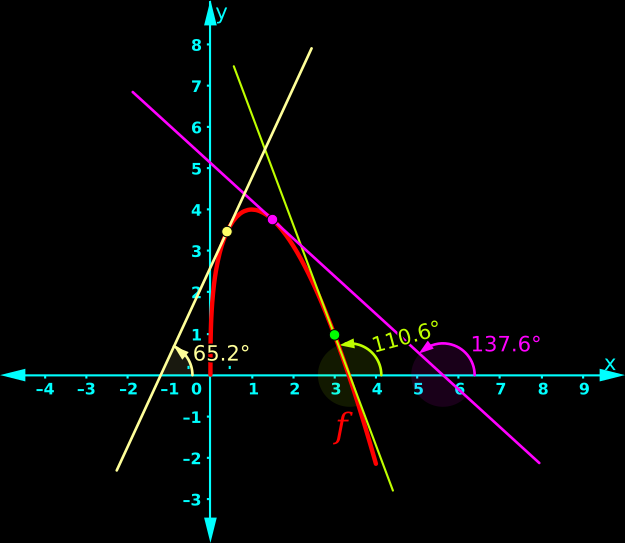
1. The red curve in fig.22.52 below shows the graph of a function f.

Fig.22.52

• We see that, the graph has an upward concavity. In such a situation, we say: f is concave up.

2. Let us analyze three random tangents of f.
Three random points are marked on f. They are: green, magenta and yellow.
• Consider the tangent at the green point.
   ♦ This tangent is drawn in green color.
   ♦ This tangent makes an angle of 110.6o with the +ve side of the x-axis.
• Consider the tangent at the magenta point.
   ♦ This tangent is drawn in magenta color.
   ♦ This tangent makes an angle of 137.6o with the +ve side of the x-axis.
• Consider the tangent at the yellow point.
   ♦ This tangent is drawn in yellow color.
   ♦ This tangent makes an angle of 65.2o with the +ve side of the x-axis.

3. We know that, slope of a line is equal to the tangent of the angle which the line makes with the +ve side of the x-axis.
• So let us write the slopes:
   ♦ Slope of green tangent = tan(110.6) = −2.66
   ♦ Slope of magenta tangent = tan(137.6) = −0.913
   ♦ Slope of yellow tangent = tan(65.2) = 2.16
• We see that:
   ♦ Magenta has a larger slope than green.
   ♦ Yellow has a larger slope than magenta.
• So the slope increases in the order:
Green < Magenta < Yellow

4. Now consider the green, magenta and yellow points.
   ♦ yellow is at the right side of magenta.
   ♦ magenta is at the right side of green.
• So we can write:
For a function which is concave up, the slope of tangent increases as we move from left to right.

5. Recall that, slope of the tangent is given by f '. This f ' is also a function.
• So, if f ' is increasing, the second derivative f '' must be +ve.
• Therefore we can write:
A function f is concave up in an interval (a,b), if f '' is +ve at all points in that interval.


Now we will see downward concavity. It can be written in 5 steps:
1.The red curve in fig.22.53 below shows the graph of a function f.

Relation between sign of second derivative and the concavity of the function.
Fig.22.53

• We see that, the graph has a downward concavity. In such a situation, we say: f is concave down.

2. Let us analyze three random tangents of f.
Three random points are marked on f. They are: yellow, magenta and green.
• Consider the tangent at the yellow point.
   ♦ This tangent is drawn in yellow color.
   ♦ This tangent makes an angle of 65.2o with the +ve side of the x-axis.
• Consider the tangent at the magenta point.
   ♦ This tangent is drawn in magenta color.
   ♦ This tangent makes an angle of 137.6o with the +ve side of the x-axis.
• Consider the tangent at the green point.
   ♦ This tangent is drawn in green color.
   ♦ This tangent makes an angle of 110.6o with the +ve side of the x-axis.

3. We know that, slope of a line is equal to the tangent of the angle which the line makes with the +ve side of the x-axis.
• So let us write the slopes:
   ♦ Slope of yellow tangent = tan(65.2) = 2.16
   ♦ Slope of magenta tangent = tan(137.6) = −0.913
   ♦ Slope of green tangent = tan(110.6) = −2.66

• We see that:
   ♦ Magenta has a smaller slope than yellow.
   ♦ Green has a smaller slope than magenta.
• So the slope decreases in the order:
Yellow < Magenta < Green

4. Now consider the green, magenta and yellow points.
   ♦ yellow is at the left side of magenta.
   ♦ magenta is at the left side of green.
• So we can write:
For a function which is concave down, the slope of tangent decreases as we move from left to right.

5. Recall that, slope of the tangent is given by f '. This f ' is also a function.
• So, if f ' is decreasing, the second derivative f '' must be −ve.
• Therefore we can write:
A function f is concave down in an interval (a,b), if f '' is −ve at all points in that interval.


Based on the above two examples, we can write the test for concavity:
Let f be a twice differentiable function in the interval (a,b).
(i) If f '' > 0 for all points in (a,b), then f is concave up.
(ii) If f '' < 0 for all points in (a,b), then f is concave down.


Now we can learn about inflection point. It can be written in 3 steps:
1. Fig.22.54 below, shows the graph of a function f.

The concavitychanges at the inflection point. The second derivative will be zero.
Fig.22.54

• We see that:
   ♦ f is concave up in the interval (a,c)
   ♦ f is concave down in the interval (c,a)
2. Let us analyze the change in sign of f '':
(i) We know that, if f is concave up, all f '' will be +ve.
• So all f '' in (a,c), will be +ve.
(ii) We also know that, if f is concave down, all f '' will be −ve.
• So all f '' in (c,a), will be −ve.
(iii) Such a change in sign for f '' is possible only if:
f '' becomes zero at some point.
(iv) Obviously, that zero point will be at the junction between "concave up portion" and "concave down portion".
• That means, f ''(c) = 0
3. So we can write the definition of inflection point:
Inflection point of a function f is the point at which f changes concavity.
4. Based on the above definition, we can write:
The inflection point in our present case is (c,f(c)).


Now we will see a solved example
Solved example 22.54
For the function f(x) = x3 − 6x2, determine all intervals where f is concave up and all intervals where f is concave down.
Solution:
Step I: Finding the inflection points and dividing the number line
1. First we will write f '(x):
f '(x) = 3x2 − 12x

2. Next we will write f ''(x):
f '' = 6x − 12

3. Equating f''(x) to zero, we get:
6x − 12 = 0
⇒ 6x = 12
⇒ x = 2

4. So the only one inflection point is at x = 2

5. Now the number line can be divided into two intervals:
(−∞,2) and (2,∞)

Step II: Finding the sign of f '' in each interval and assessing the concavity
First interval: (−∞,2)
• A convenient number in the first interval is 0.
f ''(0) = 6(0) − 12 =  −12
• Therefore, the sign of f ''(x) in the first interval is −ve.
• Then f is concave down in the first interval.

Second interval: (2,∞)
• A convenient number in the second interval is 3.
f ''(3) = 6(3) − 12 = 18 −12 = 6
• Therefore, the sign of f ''(x) in the second interval is +ve.
• Then f is concave up in the second interval.

Step III (optional): Drawing the graph

• The graph is shown in fig.22.55 below:

Fig.22.55

   ♦ f is drawn in red color.
   ♦ f ' is drawn in yellow color
   ♦ f '' is drawn in green color
• The vertical magenta dashed line divides the number line into the two intervals (−∞,2) and (2,∞). The following five facts are in agreement with our discussion on concavity test:
(i) For all inputs from the left of this vertical line, f is concave down.
(ii) For all inputs from the right of this vertical line, f is concave up.
(iii) For all inputs from the left of this vertical line, f ' is decreasing.
(iv) For all inputs from the right of this vertical line, f ' is increasing.
(v) f '' and this vertical line intersects at the x-axis. That means, value of f '' at x = 2 (the point of inflection), is zero.

Solved example 22.55
For the function f(x) = x + sin(2x), x ∈ [−π/2,π/2], determine all intervals where f is concave up and all intervals where f is concave down.
Solution:
Step I: Finding the inflection points and dividing the number line
1. First we will write f '(x):
f '(x) = 1 + 2 cos(2x)

2. Next we will write f ''(x):
f '' = −4 sin(2x)

3. Equating f''(x) to zero, we get:
−4 sin(2x) = 0
⇒ −8 sin x cos x = 0
⇒ sin x = 0 or cos x = 0
• For the equation sin x = 0, the only one solution in [−π/2,π/2], is x = 0
• For the equation cos x = 0, the only two solutions in [−π/2,π/2], are x = −π/2 and x = π/2


4. So the three inflection points are:
x = −π/2, x = 0 and x = π/2
5. Now the given domain [−π/2,π/2] can be divided into two intervals:
[−π/2,0] and [0,π/2]

Step II: Finding the sign of f '' in each interval and assessing the concavity
First interval: [−π/2,0]
• A convenient number in the first interval is −π/8.
f ''(−π/8) = −4 sin(2(−π/8))
= −4 sin (−π/4) = 4 sin (π/4) = 4/(√2) 
• Therefore, the sign of f ''(x) in the first interval is +ve.
• Then f is concave up in the first interval.

Second interval: [0,π/2]
• A convenient number in the second interval is π/8.
f ''(π/8) = −4 sin(2(π/8))
= −4 sin (π/4) = −4/(√2) 
• Therefore, the sign of f ''(x) in the second interval is −ve.
• Then f is concave down in the second interval.

Step III (optional): Drawing the graph

• The graph is shown in fig.22.56 below:

Fig.22.56
   ♦ f is drawn in red color.
   ♦ f ' is drawn in yellow color
   ♦ f '' is drawn in green color
• The two vertical magenta dashed lines are the boundaries of the domain [−π/2,π/2]. Those two vertical lines indicate the position of two inflection points x = −π/2 and x = π/2 also. Position of the third inflection point x = 0, is indicated by the y-axis. The following five facts are in agreement with our discussion on concavity test:
(i) For all inputs from between the left vertical line and y-axis, f is concave up.
(ii) For all inputs from between y-axis and the right vertical line, f is concave down.
(iii) For all inputs from between the left vertical line and y-axis, f ' is increasing.
(iv) For all inputs from between y-axis and the right vertical line, f ' is decreasing.
(v) Consider the point of intersection of  f '' with the two vertical lines and the y-axis. All those three points of intersection are at the x-axis. That means, value of f '' at those points (the points of inflection), is zero.


In the next section, we will see the second derivative test.

Previous

Contents

Next

Copyright©2024 Higher secondary mathematics.blogspot.com

Sunday, July 28, 2024

21.19 - Second Order Derivative

In the previous section, we completed a discussion on parametric functions and their differentiation. In this section, we will see second order derivative.

The basic details can be written in 4 steps:
1. Consider the function y = f(x)
• If f(x) is differentiable, then we can write:
$\rm{\frac{dy}{dx}}\,=\,f'(x)$
2. We know that, f'(x) is also a function. If this f'(x) is differentiable, we can find it’s derivative also. In such a situation, we write:
$\rm{\frac{d}{dx} \left(\frac{dy}{dx} \right)\,=\,f''(x)}$
• $\rm{f''(x)}$ is known as the second order derivative of f(x).
• $\rm{\frac{d}{dx} \left(\frac{dy}{dx} \right)}$ is denoted as $\rm{\frac{d^2 y}{dx^2}}$
• So we get: $\rm{\frac{d^2 y}{dx^2}\,=\,f''(x)}$
3. If y = f(x) then we can write in the following ways also:
• $\rm{\frac{d^2 y}{dx^2}\,=\,f''(x)\,=\,D^2 y}$
• $\rm{\frac{d^2 y}{dx^2}\,=\,f''(x)\,=\,y''}$
• $\rm{\frac{d^2 y}{dx^2}\,=\,f''(x)\,=\,y_2}$
4. We can write steps similar to the above three, to define third order derivative, fourth order derivative, fifth order derivative, so on . . .

Let us see some solved examples

Solved example 21.60
$\rm{\text{Find}~\frac{d^2 y}{dx^2}~\text{if}~y = x^3 + tan x}$.
Solution:

Example of second order derivative.
 

Solved example 21.61
If y = A sin x + B cos x, then prove that $\rm{\frac{d^2 y}{dx^2}~+~y = 0}$.
Solution:


Solved example 21.62
If y = 3e2x + 2e2x, then prove that $\rm{\frac{d^2 y}{dx^2}~-~5\frac{dy}{dx}~+~6y = 0}$.
Solution:


Solved example 21.63
If y = sin−1x, show that $\rm{(1-x^2) \frac{d^2 y}{dx^2}~-~x \frac{dy}{dx} = 0}$.
Solution:


The link below gives a few more solved examples:

Exercise 21.7


In the next section, we will see mean value theorem.

Previous

Contents


Next

Copyright©2024 Higher secondary mathematics.blogspot.com