Showing posts with label linear approximation. Show all posts

Thursday, October 24, 2024

22.11 - Change In Quantity

In the previous section, we completed a discussion on calculation of error. In this section, we will see how it can be used to find change in quantity.

The basic details can be demonstrated using an example. It can be written in 4 steps:
1. We know that, volume of a cube can be obtained using the formula: $\rm{V = l^3}$
   ♦ V is the volume of the cube.
   ♦ l is the length of side of the cube.
2. Based on the above formula, we can say that, volume is a function of length. That is.,
$\rm{V = f(l) = l^3}$
3. Consider a cube with side 5 cm.
• It's volume will be 53 = 125 cm3.
4. Suppose that, the side is increased by 2%.
• Then the new length of side = 1.02(l) = 1.02(5) = 5.1 cm
• In such a situation, there will be an increase in the volume of the cube.
• How much increase will be taking place?
Answer can be written in 4 steps:
(i) Original volume =
$\rm{V_1 \,=\, f(l_1) \,=\, {l_1}^3 \,=\, 5^3}$
(ii) New volume =
$\rm{V_2 \,=\, f(l_2) \,=\, {l_2}^3 \,=\, 5.1^3}$
(iii) So the change in volume =
$\rm{V_2 - V_1 \,=\, \Delta V \,=\, 5.1^3 ~-~5^3}$
(iv) But based on differential approximation that we learned in the previous section, we need not find the exact ΔV. we can write:
   ♦ ΔV ≈ dV (This is possible because, l2 is close to l1)
   ♦ dV = f'(l1).dl
• Thus we get:
$\begin{array}{ll} {~\color{magenta}    1    }    &{{}}    &{dV}    & {~=~}    &{f'(l_1) . dl}    \\
{~\color{magenta}    2    }    &{{}}    &{{}}    & {~=~}    &{ (3 {l_1}^2) . (l_2 - l_1)}    \\
{~\color{magenta}    3    }    &{{}}    &{{}}    & {~=~}    &{ 3({5}^2) . (5.1 - 5)}    \\
{~\color{magenta}    4    }    &{{}}    &{{}}    & {~=~}    &{3 (25) (0.1)}    \\
{~\color{magenta}    5    }    &{{}}    &{{}}    & {~=~}    &{7.5~\rm{cm^3}}    \\
\end{array}$


Let us cross check by calculating the actual change in volume ΔV.
$\rm{\Delta V \,=\, V_2 - V_1 \,=\, 5.1^3 - 5^3 \,=\,132.651 \, - \, 125 \,=\,7.651 ~ {cm}^3}$

• When we use differential approximation, we get 7.5.
• 7.5 is approximately equal to 7.651.

Solved example 22.39
Find the approximate change in the volume V of a cube of side x meters caused by increasing the side by 1%.
Solution:
1. We have:
   ♦ V = f(l) = l3
   ♦ ΔV ≈ dV (This is possible when l2 is close to l1)
   ♦ dV = f'(l1).dl
2. Original length = x m
Increased length = 1.01x m
3. Fixing l1 and l2:
l2 must be the value which causes the difficulty. So we put:
   ♦ l2 = 1.01x cm
   ♦ l1 = x cm
4. Then we get:
$\begin{array}{ll} {~\color{magenta}    1    }    &{{}}    &{dV}    & {~=~}    &{f'(l_1) . dl}    \\
{~\color{magenta}    2    }    &{{}}    &{{}}    & {~=~}    &{ (3 {l_1}^2) . (l_2 - l_1)}    \\
{~\color{magenta}    3    }    &{{}}    &{{}}    & {~=~}    &{ 3({x}^2) . (1.01x - x)}    \\
{~\color{magenta}    4    }    &{{}}    &{{}}    & {~=~}    &{3 x^2 (0.01 x)}    \\
{~\color{magenta}    5    }    &{{}}    &{{}}    & {~=~}    &{0.03 x^3~\rm{m^3}}    \\
\end{array}$

Solved example 22.40
Find the approximate change in the surface area of a cube of side x meters caused by decreasing the side by 1%.
Solution:
1. We have:
   ♦ S = f(l) = 6l2
   ♦ ΔS ≈ dS (This is possible when l2 is close to l1)
   ♦ dS = f'(l1).dl
2. Original length = x m
Decreased length = 0.99x m
3. Fixing l1 and l2:
l2 must be the value which causes the difficulty. So we put:
   ♦ l2 = 0.99x cm
   ♦ l1 = x cm
4. Then we get:
$\begin{array}{ll} {~\color{magenta}    1    }    &{{}}    &{dV}    & {~=~}    &{f'(l_1) . dl}    \\
{~\color{magenta}    2    }    &{{}}    &{{}}    & {~=~}    &{ 6( 2 l_1) . (l_2 - l_1)}    \\
{~\color{magenta}    3    }    &{{}}    &{{}}    & {~=~}    &{ 12{x} . (0.99x - x)}    \\
{~\color{magenta}    4    }    &{{}}    &{{}}    & {~=~}    &{12 x (0.01 x)}    \\
{~\color{magenta}    5    }    &{{}}    &{{}}    & {~=~}    &{0.12 x^2~\rm{m^2}}    \\
\end{array}$

Solved example 22.41
The approximate change in the volume of a cube of side x meters caused by increasing the side by 3% is
(A) 0.06 x3 m3    (B) 0.6 x3 m3    (C) 0.09 x3 m3    (B) 0.9 x3 m3
Solution:
1. We have:
   ♦ V = f(l) = l3
   ♦ ΔV ≈ dV (This is possible when l2 is close to l1)
   ♦ dV = f'(l1).dl
2. Original length = x m
Increased length = 1.03x m
3. Fixing l1 and l2:
l2 must be the value which causes the difficulty. So we put:
   ♦ l2 = 1.03x cm
   ♦ l1 = x cm
4. Then we get:
$\begin{array}{ll} {~\color{magenta}    1    }    &{{}}    &{dV}    & {~=~}    &{f'(l_1) . dl}    \\
{~\color{magenta}    2    }    &{{}}    &{{}}    & {~=~}    &{ (3 {l_1}^2) . (l_2 - l_1)}    \\
{~\color{magenta}    3    }    &{{}}    &{{}}    & {~=~}    &{ 3({x}^2) . (1.03x - x)}    \\
{~\color{magenta}    4    }    &{{}}    &{{}}    & {~=~}    &{3 x^2 (0.03 x)}    \\
{~\color{magenta}    5    }    &{{}}    &{{}}    & {~=~}    &{0.09 x^3~\rm{m^3}}    \\
\end{array}$

5. So the correct option is (C)


The link below gives a few more solved examples:

Exercise 22.4


In the next section, we will see Maxima and Minima.

Previous

Contents

Next

Copyright©2024 Higher secondary mathematics.blogspot.com

Wednesday, October 23, 2024

22.10 - Calculating The Amount of Error

In the previous section, we completed a discussion on differential approximation. In this section, we will see how it can be used to find amount of error.

The basic details can be demonstrated using an example. It can be written in 6 steps:
1. We know that, volume of a sphere can be obtained using the formula: $\rm{V = \frac{4}{3} \pi r^3}$
   ♦ V is the volume of the sphere.
   ♦ r is the radius of the sphere.
2. Based on the above formula, we can say that, volume is a function of radius. That is.,
$\rm{V = f(r) = \frac{4}{3} \pi r^3}$
3. Suppose that, the radius of a sphere is measured to be 5 cm with an error of 0.1 cm.
• Then the actual radius r will be such that:
4.9 ≤ r ≤ 5.1
4. Consider the situation:
   ♦ The actual radius is 5.1 cm.
   ♦ We use 5 cm for calculating the volume.
• In such a situation, there will be error in the calculated volume.
• How much error will be present in the calculated volume?
Answer can be written in 4 steps:
(i) Calculated volume =
$\rm{V_1 \,=\, f(r_1) \,=\, \frac{4}{3} \pi {r_1}^3 \,=\, \frac{4}{3} \pi (5^3)}$
(ii) Actual volume =
$\rm{V_2 \,=\, f(r_2) \,=\, \frac{4}{3} \pi {r_2}^3 \,=\, \frac{4}{3} \pi ({5.1}^3)}$
(iii) So the error in the calculated volume =
$\rm{V_2 - V_1 \,=\, \Delta V \,=\, \frac{4}{3} \pi ({5.1}^3) ~-~\frac{4}{3} \pi ({5}^3)}$
(iv) But based on differential approximation that we learned in the previous section, we need not find the exact ΔV. we can write:
   ♦ ΔV ≈ dV (This is possible because, r2 is close to r1)
   ♦ dV = f'(r1).dr
• Thus we get:
$\begin{array}{ll} {~\color{magenta}    1    }    &{{}}    &{dV}    & {~=~}    &{f'(r_1) . dr}    \\
{~\color{magenta}    2    }    &{{}}    &{{}}    & {~=~}    &{\frac{4}{3} \pi (3 {r_1}^2) . (r_2 - r_1)}    \\
{~\color{magenta}    3    }    &{{}}    &{{}}    & {~=~}    &{4 \pi  (5^2) . (5.1 - 5)}    \\
{~\color{magenta}    4    }    &{{}}    &{{}}    & {~=~}    &{4 \pi  (25) . (0.1)}    \\
{~\color{magenta}    5    }    &{{}}    &{{}}    & {~=~}    &{10 \pi~\rm{cm^3}}    \\
\end{array}$
5. Consider the situation:
   ♦ The actual radius is 4.9 cm.
   ♦ We use 5 cm for calculating the volume.
• In such a situation also, there will be error in the calculated volume.
• How much error will be present in the calculated volume?
Answer can be written in 4 steps:
(i) Calculated volume =
$\rm{V_1 \,=\, f(r_1) \,=\, \frac{4}{3} \pi {r_1}^3 \,=\, \frac{4}{3} \pi (5^3)}$
(ii) Actual volume =
$\rm{V_2 \,=\, f(r_2) \,=\, \frac{4}{3} \pi {r_2}^3 \,=\, \frac{4}{3} \pi ({4.9}^3)}$
(iii) So the error in the calculated volume =
$\rm{V_2 - V_1 \,=\, \Delta V \,=\, \frac{4}{3} \pi ({4.9}^3) ~-~\frac{4}{3} \pi ({5}^3)}$
(iv) But based on differential approximation that we learned in the previous section, we need not find the exact ΔV. we can write:
   ♦ ΔV ≈ dV (This is possible because, r2 is close to r1)
   ♦ dV = f'(r1).dr
• Thus we get:
$\begin{array}{ll} {~\color{magenta}    1    }    &{{}}    &{dV}    & {~=~}    &{f'(r_1) . dr}    \\
{~\color{magenta}    2    }    &{{}}    &{{}}    & {~=~}    &{\frac{4}{3} \pi (3 {r_1}^2) . (r_2 - r_1)}    \\
{~\color{magenta}    3    }    &{{}}    &{{}}    & {~=~}    &{4 \pi  (5^2) . (4.9 - 5)}    \\
{~\color{magenta}    4    }    &{{}}    &{{}}    & {~=~}    &{4 \pi  (25) . (-0.1)}    \\
{~\color{magenta}    5    }    &{{}}    &{{}}    & {~=~}    &{-10 \pi~\rm{cm^3}}    \\
\end{array}$
6. So we can write:
The error (dV) in calculated volume will be such that:
−10π ≤ dV ≤ 10π.


Let us cross check by calculating ΔV
• Consider the situation:
   ♦ The actual radius is 5.1 cm.
   ♦ We use 5 cm for calculating the volume.
Then we get:
$\begin{array}{ll} {~\color{magenta}    1    }    &{{}}    &{\Delta V}    & {~=~}    &{V_2 - V_1}    \\
{~\color{magenta}    2    }    &{{}}    &{{}}    & {~=~}    &{\frac{4}{3} \pi ({5.1}^3)~-~\frac{4}{3} \pi ({5}^3)}    \\
{~\color{magenta}    3    }    &{{}}    &{{}}    & {~=~}    &{10.2013333333333 \pi ~\rm{cm^3}}    \\
\end{array}$

• Consider the situation:
   ♦ The actual radius is 5.1 cm.
   ♦ We use 5 cm for calculating the volume.
Then we get:
$\begin{array}{ll} {~\color{magenta}    1    }    &{{}}    &{\Delta V}    & {~=~}    &{V_2 - V_1}    \\
{~\color{magenta}    2    }    &{{}}    &{{}}    & {~=~}    &{\frac{4}{3} \pi ({4.9}^3)~-~\frac{4}{3} \pi ({5}^3)}    \\
{~\color{magenta}    3    }    &{{}}    &{{}}    & {~=~}    &{-9.80133333333329 \pi ~\rm{cm^3}}    \\
\end{array}$

• When we use differential approximation, we get 10π and −10π.
• 10π is approximately equal to 10.2013 π.
• −10π is approximately equal to −9.8013333 π.

Solved example 22.37
If the radius of a sphere is measured as 9 cm with an error of 0.03 cm, then find the approximate error in calculating its volume. 
Solution:
1. The actual radius r will be such that:
8.97 ≤ r ≤ 9.03
2. Consider the situation:
   ♦ The actual radius is 9.03 cm.
   ♦ We use 9 cm for calculating the volume.
3. First we fix r1 and r2:
r2 must be the value which causes the difficulty. So we put:
   ♦ r2 = 9.03 cm
   ♦ r1 = 9.0 cm
4. Then we get:
$\begin{array}{ll} {~\color{magenta}    1    }    &{{}}    &{dV}    & {~=~}    &{f'(r_1) . dr}    \\
{~\color{magenta}    2    }    &{{}}    &{{}}    & {~=~}    &{\frac{4}{3} \pi (3 {r_1}^2) . (r_2 - r_1)}    \\
{~\color{magenta}    3    }    &{{}}    &{{}}    & {~=~}    &{4 \pi  (9^2) . (9.03 - 9)}    \\
{~\color{magenta}    4    }    &{{}}    &{{}}    & {~=~}    &{4 \pi  (81) . (0.03)}    \\
{~\color{magenta}    5    }    &{{}}    &{{}}    & {~=~}    &{9.72 \pi~\rm{cm^3}}    \\
\end{array}$
5. Consider the situation:
   ♦ The actual radius is 8.97 cm.
   ♦ We use 9 cm for calculating the volume.
• Here we get the same result with opposite sign because dx is the same value but with opposite sign.
• That means, dV in this case is −9.72π cm3.
6. We can write:
The error (dV) in calculated volume will be such that:
−9.72π ≤ dV ≤ 9.72π.

Solved example 22.38
If the length of a cube is measured as 6 cm with an error of 0.2 cm, then find the approximate error in calculating its volume. 
Solution:
1. The actual length (l) will be such that:
5.8 ≤ l ≤ 6.2
2. Consider the situation:
   ♦ The actual length is 6.2 cm.
   ♦ We use 6 cm for calculating the volume.
3. First we fix l1 and l2:
l2 must be the value which causes the difficulty. So we put:
   ♦ l2 = 6.2 cm
   ♦ l1 = 6.0 cm
4. Then we get:
$\begin{array}{ll} {~\color{magenta}    1    }    &{{}}    &{dV}    & {~=~}    &{f'(l_1) . dl}    \\
{~\color{magenta}    2    }    &{{}}    &{{}}    & {~=~}    &{ (3 {l_1}^2) . (l_2 - l_1)}    \\
{~\color{magenta}    3    }    &{{}}    &{{}}    & {~=~}    &{3  (6^2) . (6.2 - 6)}    \\
{~\color{magenta}    4    }    &{{}}    &{{}}    & {~=~}    &{3 (36) . (0.2)}    \\
{~\color{magenta}    5    }    &{{}}    &{{}}    & {~=~}    &{21.6~\rm{cm^3}}    \\
\end{array}$
5. Consider the situation:
   ♦ The actual length is 5.8 cm.
   ♦ We use 6 cm for calculating the volume.
• Here we get the same result with opposite sign because dx is the same value but with opposite sign.
• That means, dV in this case is −21.6 cm3.
6. We can write:
The error (dV) in calculated volume will be such that:
−21.6 ≤ dV ≤ 21.6.


In the next section, we will see change in quantity.

Previous

Contents

Next

Copyright©2024 Higher secondary mathematics.blogspot.com

Friday, October 18, 2024

22.7 - Solved Examples on Linear Approximation

In the previous section, we saw the basics about linear approximation. We saw some solved examples also. In this section, we will see a few more solved examples.

Solved example 22.24
Write the linear approximation of f(x) = x1/3 and use it to estimate 251/3.
Solution:
1. Given $\rm{f(x) = x^{1/3}}$
• We are asked to write the linear approximation of this function at an arbitrary point. Let us choose the arbitrary point x = a.
2. The slope at any point is $f'(x) ~=~\rm{\frac{1}{3} (x)^{-2/3}}$  
• So the slope at 'a' is $\rm{f'(a) ~=~\frac{1}{3} (a)^{-2/3}}$
3. At the point where x = a, the y coordinate can be calculated as follows:
$\rm{y = x^{1/3}= a^{1/3}}$
4. So the tangent at x = a can be obtained as:
$\begin{array}{ll} {~\color{magenta}    1    }    &{{}}    &{y - a^{1/3}}    & {~=~}    &{\frac{1}{3} a^{-2/3} (x - a)}    \\
{~\color{magenta}    2    }    &{\implies}    &{y}    & {~=~}    &{\frac{1}{3} a^{-2/3} (x - a)~+~a^{1/3}}    \\
\end{array}$
5. So the linear approximation of f at x = a is:
$L(x) = \frac{1}{3} a^{-2/3} (x - a)~+~a^{1/3}$
6. Using linear approximation, we can calculate f(b) because:
f(b) ≈ L(b) if b is close to a.
• In our present case, b = 25
• 'a' should be selected in such a way that:
   ♦ 'a' is a convenient number
   ♦ 'a' is close to 'b'.
• We can take a = 27
Cube root of 27 is already known. So it is a convenient number. Also, 27 is close to 25
7. Based on the result in (5), we can write:
Linear approximation of f at x = 27 is:
$\begin{array}{ll} {~\color{magenta}    1    }    &{{}}    &{L(x)}    & {~=~}    &{\frac{1}{3} a^{-2/3} (x - a)~+~a^{1/3}}    \\
{~\color{magenta}    2    }    &{\implies}    &{L(x)_{a=27}}    & {~=~}    &{\frac{1}{3} (27^{-2/3}) (x - 27)~+~27^{1/3}}    \\
{~\color{magenta}    3    }    &{{}}    &{{}}    & {~=~}    &{\frac{1}{3} (3^{-2}) (x - 27)~+~3}    \\
{~\color{magenta}    4    }    &{{}}    &{{}}    & {~=~}    &{(3^{-3}) (x - 27)~+~3}    \\
\end{array}$
8. Based on what we wrote in (6), we get:
$\begin{array}{ll} {~\color{magenta}    1    }    &{{}}    &{f(b)}    & {~≈~}    &{L(b)}    \\
{~\color{magenta}    2    }    &{\implies}    &{f(25)}    & {~≈~}    &{L(25)}    \\
{~\color{magenta}    3    }    &{\implies}    &{25^{1/3}}    & {~≈~}    &{(3^{-3}) (25 - 27)~+~3}    \\
{~\color{magenta}    4    }    &{{}}    &{{}}    & {~≈~}    &{\frac{-2}{27}~+~3}    \\
{~\color{magenta}    5    }    &{{}}    &{{}}    & {~≈~}    &{2.9259259}    \\
\end{array}$
9. It is interesting to note that, if we use a calculator or computer to calculate the cube root of 25, we will get:
$25^{1/3}~=~2.9240177$

Solved example 22.25
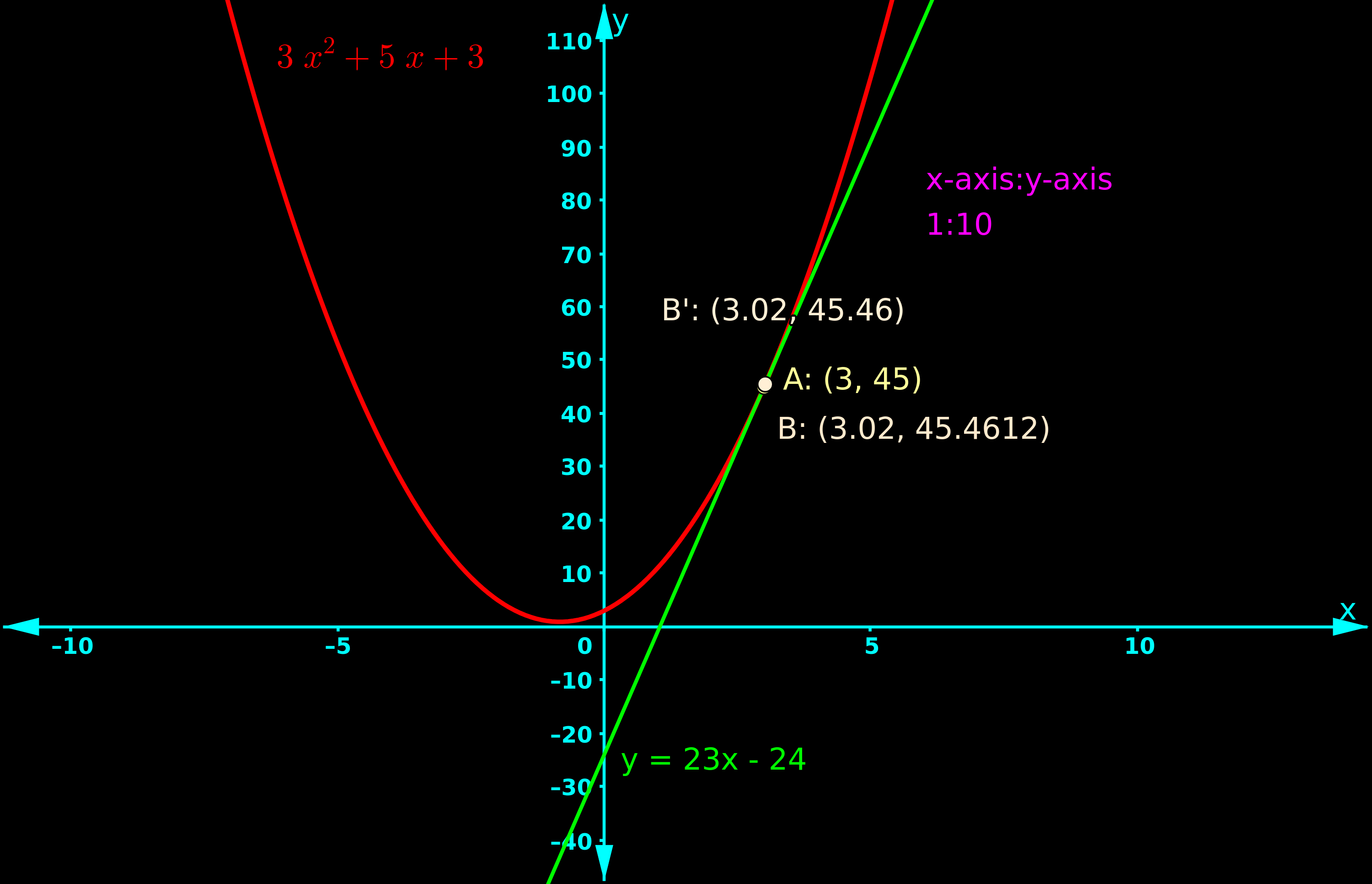
Find the approximate value of f(3.02) where
f(x) = 3x2 + 5x + 3.
Solution:
1. Given f(x) = 3x2 + 5x + 3
• We will first write the linear approximation of this function at an arbitrary point. Let us choose the arbitrary point x = a.
2. The slope at any point is f'(x) = 6x + 5
• So the slope at 'a' is f'(a) = 6a + 5
3. At the point where x = a, the y coordinate can be calculated as follows:
y = 3x2 + 5x + 3 = 3a2 + 5a + 3
4. So the tangent at x = a can be obtained as:
$\begin{array}{ll} {~\color{magenta}    1    }    &{{}}    &{y - (3a^2 + 5a + 3)}    & {~=~}    &{(6a+5) (x - a)}    \\
{~\color{magenta}    2    }    &{\implies}    &{y}    & {~=~}    &{(6a+5) (x - a)~+~(3a^2 + 5a + 3)}    \\
\end{array}$
5. So the linear approximation of f at x = a is:
$L(x) = (6a+5) (x - a)~+~(3a^2 + 5a + 3)$
6. Using linear approximation, we can calculate f(b) because:
f(b) ≈ L(b) if b is close to a.
• In our present case, b = 3.02
• 'a' should be selected in such a way that:
   ♦ 'a' is a convenient number
   ♦ 'a' is close to 'b'.
• We can take a = 3
'3' is a whole number which makes the calculations easy. So it is a convenient number. Also, 3 is close to 3.02
7. Based on the result in (5), we can write:
Linear approximation of f at x = 3 is:
$\begin{array}{ll} {~\color{magenta}    1    }    &{{}}    &{L(x)}    & {~=~}    &{(6a+5) (x - a)~+~(3a^2 + 5a + 3)}    \\
{~\color{magenta}    2    }    &{\implies}    &{L(x)_{a=3}}    & {~=~}    &{(18+5) (x - 3)~+~(27 + 15 + 3)}    \\
{~\color{magenta}    3    }    &{{}}    &{{}}    & {~=~}    &{(23) (x - 3)~+~(45)}    \\
\end{array}$
8. Based on what we wrote in (6), we get:
$\begin{array}{ll} {~\color{magenta}    1    }    &{{}}    &{f(b)}    & {~≈~}    &{L(b)}    \\
{~\color{magenta}    2    }    &{\implies}    &{f(3.02)}    & {~≈~}    &{L(3.02)}    \\
{~\color{magenta}    3    }    &{}    &{}    & {~≈~}    &{(23) (3.02 - 3)~+~(45)}    \\
{~\color{magenta}    4    }    &{{}}    &{{}}    & {~≈~}    &{(23) (0.02)~+~(45)}    \\
{~\color{magenta}    5    }    &{{}}    &{{}}    & {~≈~}    &{45.46}    \\
\end{array}$
9. It is interesting to note that, if we use a calculator or computer to calculate the given function at 3.02, we will get:
f(x) = 3(3.02)2 + 5(3.02) + 3 = 45.4612
10. Fig.22.23 below shows the graph.
   ♦ f is drawn in red color
   ♦ L is drawn in green color

Fig.22.23

   ♦ A is a point on f
   ♦ B is a point on f
   ♦ B' is a point on L
• We want the y-coordinate at B. But, for ease of calculation, we use linear approximation and obtain the y-coordinate at B'.
• In the graph, A, B and B' are so close to each other that, they are not distinctly visible from each other.


Solved example 22.26
Write the linear approximation of f(x) = sin x and use it to estimate sin 62o.
Solution:
1. Given $\rm{f(x) = \sin x}$
• We are asked to write the linear approximation of this function at an arbitrary point. Let us choose the arbitrary point x = a.
2. The slope at any point is $\rm{f'(x) ~=~\cos x}$  
• So the slope at 'a' is $\rm{f'(a) ~=~\cos a}$
3. At the point where x = a, the y coordinate can be calculated as follows:
y = sin x = sin a
4.  So the tangent at x = a can be obtained as:
$\begin{array}{ll} {~\color{magenta}    1    }    &{{}}    &{y - \sin a}    & {~=~}    &{\cos a \,(x - a)}    \\
{~\color{magenta}    2    }    &{\implies}    &{y}    & {~=~}    &{\cos a \, (x - a) + \sin a}    \\
{~\color{magenta}    3    }    &{{}}    &{{}}    & {~=~}    &{x \cos a ~-~ a \cos a ~+~\sin a}    \\
\end{array}$
5. So the linear approximation of f at x = a is:
$L(x) = x \cos a ~-~ a \cos a ~+~\sin a$
6. Using linear approximation, we can calculate f(b) because:
f(b) ≈ L(b) if b is close to a.
• In our present case, b = 62o.
• Converting this to radians, we get:
$\rm{62^o ~=~62 \times \frac{\pi}{180}~=~\frac{62 \pi}{180}}$
• 'a' should be selected in such a way that:
   ♦ 'a' is a convenient number
   ♦ 'a' is close to 'b'.
• We can take a = 60o
cosine and sine of 60 is already known. So it is a convenient number. Also, 60 is close to 62.
• Converting 60o to radians, we have:
$\rm{60^o ~=~\frac{\pi}{3}}$
7. Based on the result in (5), we can write:
Linear approximation of f at x = π/3 is:
$\begin{array}{ll} {~\color{magenta}    1    }    &{{}}    &{L(x)}    & {~=~}    &{x \cos a ~-~ a \cos a ~+~\sin a}    \\
{~\color{magenta}    2    }    &{\implies}    &{L(x)_{a=\pi / 3}}    & {~=~}    &{x \cos \frac{\pi}{3} ~-~ a \cos \frac{\pi}{3} ~+~\sin \frac{\pi}{3}}    \\
{~\color{magenta}    3    }    &{{}}    &{{}}    & {~=~}    &{\frac{x}{2} ~-~ \frac{\pi}{6} ~+~ \frac{\sqrt3}{2}}    \\
\end{array}$
8. Based on what we wrote in (6), we get:
$\begin{array}{ll} {~\color{magenta}    1    }    &{{}}    &{f(b)}    & {~≈~}    &{L(b)}    \\
{~\color{magenta}    2    }    &{\implies}    &{f(\frac{62 \pi}{180})}    & {~≈~}    &{L(\frac{62 \pi}{180})}    \\
{~\color{magenta}    3    }    &{\implies}    &{\sin \frac{62 \pi}{180}}    & {~≈~}    &{\frac{62 \pi}{180} ~-~ \frac{\pi}{6} ~+~ \frac{\sqrt3}{2}}    \\
{~\color{magenta}    4    }    &{{}}    &{{}}    & {~≈~}    &{0.883478
}    \\
\end{array}$
9. It is interesting to note that, if we use a calculator or computer to calculate the sine of 62o, we will get:
$\sin 62^o~=~0.882947$

Solved example 22.27
Write the linear approximation of f(x) = cos x and use it to estimate cos 89o.
Solution:
1. Given $\rm{f(x) = \cos x}$
• We are asked to write the linear approximation of this function at an arbitrary point. Let us choose the arbitrary point x = a.
2. The slope at any point is $\rm{f'(x) ~=~-\sin x}$  
• So the slope at 'a' is $\rm{f'(a) ~=~-\sin a}$
3. At the point where x = a, the y coordinate can be calculated as follows:
y = cos x = cos a
4.  So the tangent at x = a can be obtained as:
$\begin{array}{ll} {~\color{magenta}    1    }    &{{}}    &{y - \cos a}    & {~=~}    &{-\sin a \,(x - a)}    \\
{~\color{magenta}    2    }    &{\implies}    &{y}    & {~=~}    &{-\sin a \, (x - a) + \cos a}    \\
{~\color{magenta}    3    }    &{{}}    &{{}}    & {~=~}    &{-x \sin a ~+~ a \sin a ~+~\cos a}    \\
\end{array}$
5. So the linear approximation of f at x = a is:
$L(x) = -x \sin a ~+~ a \sin a ~+~\cos a$
6. Using linear approximation, we can calculate f(b) because:
f(b) ≈ L(b) if b is close to a.
• In our present case, b = 89o.
• Converting this to radians, we get:
$\rm{89^o ~=~89 \times \frac{\pi}{180}~=~\frac{89 \pi}{180}}$
• 'a' should be selected in such a way that:
   ♦ 'a' is a convenient number
   ♦ 'a' is close to 'b'.
• We can take a = 90o
cosine and sine of 90 is already known. So it is a convenient number. Also, 90 is close to 89.
• Converting 90o to radians, we have:
$\rm{90^o ~=~\frac{\pi}{2}}$
7. Based on the result in (5), we can write:
Linear approximation of f at x = π/2 is:
$\begin{array}{ll} {~\color{magenta}    1    }    &{{}}    &{L(x)}    & {~=~}    &{-x \sin a ~+~ a \sin a ~+~\cos a}    \\
{~\color{magenta}    2    }    &{\implies}    &{L(x)_{a=\pi / 2}}    & {~=~}    &{-x \sin \frac{\pi}{2} ~+~ a \sin \frac{\pi}{2} ~+~\cos \frac{\pi}{2}}    \\
{~\color{magenta}    3    }    &{{}}    &{{}}    & {~=~}    &{-x ~+~ \frac{\pi}{2}}    \\
\end{array}$
8. Based on what we wrote in (6), we get:
$\begin{array}{ll} {~\color{magenta}    1    }    &{{}}    &{f(b)}    & {~≈~}    &{L(b)}    \\
{~\color{magenta}    2    }    &{\implies}    &{f(\frac{89 \pi}{180})}    & {~≈~}    &{L(\frac{89 \pi}{180})}    \\
{~\color{magenta}    3    }    &{\implies}    &{\cos \frac{89 \pi}{180}}    & {~≈~}    &{-\frac{89 \pi}{180} ~+~ \frac{\pi}{2}}    \\
{~\color{magenta}    4    }    &{{}}    &{{}}    & {~≈~}    &{0.01745329}    \\
\end{array}$
9. It is interesting to note that, if we use a calculator or computer to calculate the cosine of 89o, we will get:
$\cos 89^o~=~0.017452406$

Solved example 22.28
Write the linear approximation of f(x) = (1+x)n and use it to estimate (1.01)3.
Solution:
1. Given $\rm{f(x) = (1+x)^n}$
• We are asked to write the linear approximation of this function at an arbitrary point. Let us choose the arbitrary point x = a.
2. The slope at any point is $\rm{f'(x) ~=~n(1+x)^{n-1}}$  
• So the slope at 'a' is $\rm{f'(a) ~=~n(1+a)^{n-1}}$
3. At the point where x = a, the y coordinate can be calculated as follows:
$\rm{y = (1+a)^n}$
4.  So the tangent at x = a can be obtained as:
$\begin{array}{ll} {~\color{magenta}    1    }    &{{}}    &{y - (1+a)^n}    & {~=~}    &{n(1+a)^{n-1} \,(x - a)}    \\
{~\color{magenta}    2    }    &{\implies}    &{y}    & {~=~}    &{nx(1+a)^{n-1}~-~na(1+a)^{n-1}~+~(1+a)^{n}}    \\
\end{array}$
5. So the linear approximation of f at x = a is:
$L(x) = nx(1+a)^{n-1}~-~na(1+a)^{n-1}~+~(1+a)^{n}$
6. Using linear approximation, we can calculate f(b) because:
f(b) ≈ L(b) if b is close to a.
• In our present case, b = 0.01.
• 'a' should be selected in such a way that:
   ♦ 'a' is a convenient number
   ♦ 'a' is close to 'b'.
• We can take a = 0
Then (1+a) will become 1. So it is a convenient number. Also, 0 is close to 0.01.
7. Based on the result in (5), we can write:
Linear approximation of f at x = 0 is:
$\begin{array}{ll} {~\color{magenta}    1    }    &{{}}    &{L(x)}    & {~=~}    &{nx(1+a)^{n-1}~-~na(1+a)^{n-1}~+~(1+a)^{n}}    \\
{~\color{magenta}    2    }    &{\implies}    &{L(x)_{a=0}}    & {~=~}    &{nx(1) ~-~n(0)(1)~+~1}    \\
{~\color{magenta}    3    }    &{{}}    &{{}}    & {~=~}    &{nx ~+~ 1}    \\
\end{array}$
8. Based on what we wrote in (6), we get:
$\begin{array}{ll} {~\color{magenta}    1    }    &{{}}    &{f(b)}    & {~≈~}    &{L(b)}    \\
{~\color{magenta}    2    }    &{\implies}    &{f(0.01)}    & {~≈~}    &{L(0.01)}    \\
{~\color{magenta}    3    }    &{\implies}    &{(1+0.01)^n}    & {~≈~}    &{n(0.01) + 1}    \\
{~\color{magenta}    4    }    &{{\implies}}    &{{(1.01)^3}}    & {~≈~}    &{3(0.01) + 1}    \\
{~\color{magenta}    5    }    &{{}}    &{{}}    & {~≈~}    &{1.03}    \\
\end{array}$
9. It is interesting to note that, if we use a calculator or computer to calculate (1.01)3, we will get:
$(1.01)^3~=~1.030301$

Solved example 22.29
Write the linear approximation of f(x) = (1−x)1/10 and use it to estimate (0.999)1/10.
Solution:
1. Given $\rm{f(x) = (1-x)^{1/10}}$
• We are asked to write the linear approximation of this function at an arbitrary point. Let us choose the arbitrary point x = a.
2. The slope at any point is:
$\rm{f'(x) ~=~\frac{1}{10}(1- x)^{-9/10} (-1)~=~\frac{-1}{10}(1- x)^{-9/10}}$  
• So the slope at 'a' is $\rm{f'(a) ~=~\frac{-1}{10}(1- a)^{-9/10}}$
3. At the point where x = a, the y coordinate can be calculated as follows:
$\rm{y = (1-a)^{1/10}}$
4.  So the tangent at x = a can be obtained as:
$\begin{array}{ll} {~\color{magenta}    1    }    &{{}}    &{y - (1-a)^{1/10}}    & {~=~}    &{\frac{-1}{10}(1- a)^{-9/10} \,(x - a)}    \\
{~\color{magenta}    2    }    &{\implies}    &{y}    & {~=~}    &{\frac{-1}{10}(1- a)^{-9/10} \,(x - a)~+~(1-a)^{1/10}}    \\
\end{array}$
5. So the linear approximation of f at x = a is:
$L(x) = \frac{-1}{10}(1- a)^{-9/10} \,(x - a)~+~(1-a)^{1/10}$
6. Using linear approximation, we can calculate f(b) because:
f(b) ≈ L(b) if b is close to a.
• In our present case, b = 0.001.
This is because, 0.999 = (1 − 0.001)
• 'a' should be selected in such a way that:
   ♦ 'a' is a convenient number
   ♦ 'a' is close to 'b'.
• We can take a = 0
Then (1−a) will become 1. So it is a convenient number. Also, 0 is close to 0.001.
7. Based on the result in (5), we can write:
Linear approximation of f at x = 0 is:
$\begin{array}{ll} {~\color{magenta}    1    }    &{{}}    &{L(x)}    & {~=~}    &{\frac{-1}{10}(1- a)^{-9/10} \,(x - a)~+~(1-a)^{1/10}}    \\
{~\color{magenta}    2    }    &{\implies}    &{L(x)_{a=0}}    & {~=~}    &{\frac{-1}{10}(1) \,(x)~+~1}    \\
{~\color{magenta}    3    }    &{{}}    &{{}}    & {~=~}    &{\frac{-x}{10} ~+~ 1}    \\
\end{array}$
8. Based on what we wrote in (6), we get:
$\begin{array}{ll} {~\color{magenta}    1    }    &{{}}    &{f(b)}    & {~≈~}    &{L(b)}    \\
{~\color{magenta}    2    }    &{\implies}    &{f(0.001)}    & {~≈~}    &{L(0.001)}    \\
{~\color{magenta}    3    }    &{\implies}    &{(1-0.001)^{1/10}}    & {~≈~}    &{\frac{-0.001}{10} + 1}    \\
{~\color{magenta}    4    }    &{{\implies}}    &{{(0.999)^{1/10}}}    & {~≈~}    &{-0.0001 + 1}    \\
{~\color{magenta}    5    }    &{{}}    &{{}}    & {~≈~}    &{0.9999}    \\
\end{array}$
9. It is interesting to note that, if we use a calculator or computer to calculate (0.999)1/10, we will get:
$(0.999)^{1/10}~=~0.9998999$
10. Fig.22.24 below shows the graph.
   ♦ f is drawn in red color
   ♦ L is drawn in green color

Fig.22.24
   ♦ A is a point on f
   ♦ B is a point on f
   ♦ B' is a point on L
• We want the y-coordinate at B. But, for ease of calculation, we use linear approximation and obtain the y-coordinate at B'.
• In the graph, A, B and B' are so close to each other that, they are not distinctly visible from each other.

In the next section, we will see Differentials.

Previous

Contents

Next

Copyright©2024 Higher secondary mathematics.blogspot.com

Wednesday, October 16, 2024

22.6 - Linear Approximation

In the previous section, we completed a discussion on Tangents and Normals. In this section, we will see Approximations.

Some basic details can be written in 12 steps:
1. Fig.22.21 below shows the graph of f(x) = x3 − 6x + 2
It is drawn in red color.

Fig.22.21


2. Consider point A where x = 2
We get: f(2) = (2)3 − 6(2) + 2 = −2
3. The green line is the tangent at x = 2
• Let us find the equation of this tangent.
f'(x) = 3x2` − 6
⇒ f'(2) = 3(2)2` − 6 = 6
y − (−2) = 6(x − 2)
⇒ y + 2 = 6 x − 12
⇒ y = 6x − 14
4. This tangent can be considered as a function of x. We will name this function as L. So we can write:
L(x) = 6x − 14
5. Let us calculate the value of L at x = 2
L(2) = 6(2) − 14 = −2
6. From (2) and (5), we can write: f(2) = L(2)
• In general, we can write: f(a) = L(a)
This is possible because, the tangent L is drawn at x = a
7. Consider another point B where x = 1.9.
    ♦ At A, x = 2
    ♦ At B, x = 1.9
• So we can say that, B is close to A
    ♦ f(1.9) = (1.9)3 − 6(1.9) + 2 = −2.541
    ♦ L(1.9) = 6(1.9) − 14 = −2.6
• We see that, f(1.9) is approximately equal to L(1.9)
• When we calculate L(1.9), we get the coordinates of a new point as (1.9, − 2.6). We will name this point as B'.
In the graph, we see that, B is very close to B'.
8. From the above discussion, we can write 3 points:
(i) We wanted the value of f at B. For that, we used the tangent at A
(ii) If we directly use f, we get: f(1.9) = −2.541
(iii) If we use the tangent at A, we get: L(1.9) = −2.6
(iv) We can write: f(1.9) ≈ L(1.9)
9. We accept the fact that, there is considerable difference between −2.541 and −2.6
• This difference is due to the fact that, B is not very close to A.
    ♦ x value at B is 1.9
    ♦ x value at A is 2
• If B is very close to A, we will get better approximations. Let us try such values for B:
(i) At B, if x = 1.95, we get:
f(1.95) = −2.2851 and L(1.95) = −2.3
(ii) At B, if x = 1.98, we get:
f(1.98) = −2.1176 and L(1.98) = −2.12
(iii) At B, if x = 1.99, we get:
f(1.99) = −2.059401 and L(1.99) = −2.06
(iv) At B, if x = 1.999, we get:
f(1.999) = −2.005994001 and L(1.999) = −2.006
(iv) At B, if x = 1.9999, we get:
f(1.9999) = −2.000599940001 and L(1.999) = −2.0006
10. It is clear that, if B is very close to A, then the tangent at A can be used to find the approximate value of f at B.
• The method can be summarized in 6 steps:
(i) We want the approximate value of f at B. Assume that, at B, x = b.
• So we want the approximate value of f(b).
(ii) For that, we choose a convenient point A, which is very close to B.
• Assume that, at A, x = a
(iii) We write the function L at A.
(iv) Then the approximate value of f(b) will be L(b)
(v) In the function f, the power of x may be one, two or above. But in the function L, the power of x will be always one. So it is easier to find L(b) than to find f(b).
(vi) The function L is known by three different names. We can use any on of them
   ♦ L is called linear approximation of f at x = a.
   ♦ L is called tangent line approximation of f at x = a.
   ♦ L is called linearization of f at x = a.
11. This method will work also when B (very close to A), is to the right of A. Let us see such points.
(i) At B, if x = 2.05, we get:
f(2.05) = −1.6848 and L(2.05) = −1.7
(ii) At B, if x = 2.02, we get:
f(2.02) = −1.877592 and L(2.02) = −1.88
(iii) At B, if x = 2.01, we get:
f(2.01) = −-1.939399 and L(2.01) = −1.94
(iv) At B, if x = 2.001, we get:
f(2.001) = −-1.993993999 and L(2.001) = −1.994
(iv) At B, if x = 2.0001, we get:
f(2.0001) = −1.999399939999 and L(2.0001) = −1.9994
12. This method will work only if B is very close to A. In the fig.22.21 above, a point C is marked. This point C is not close to A.
    ♦ x value at C is 2.4
    ♦ x value at A is 2
• We see that:
    ♦ f(2.4) is 1.424
    ♦ L(2.4) = 0.4
• There is a very large difference between 1.424 and 0.4
• This is because, there is a large difference between 2 and 2.4.


Let us see some solved examples:

Solved example 22.21
Write the linear approximation of f(x) = √x and use it to estimate $\sqrt{36.6}$.
Solution:
1. Given $\rm{f(x) = \sqrt{x}}$
• We are asked to write the linear approximation of this function at an arbitrary point. Let us choose the arbitrary point x = a.
2. The slope at any point is $f'(x) ~=~\rm{\frac{1}{2} (x)^{-1/2}}$  
• So the slope at 'a' is $\rm{f'(a) ~=~\frac{1}{2} (a)^{-1/2}~=~\frac{1}{2 \sqrt{a}}}$
3. At the point where x = a, the y coordinate can be calculated as follows:
y = √x = √a
4. So the tangent at x = a can be obtained as:
$\begin{array}{ll} {~\color{magenta}    1    }    &{{}}    &{y - \sqrt{a}}    & {~=~}    &{\frac{1}{2 \sqrt{a}} (x - a)}    \\
{~\color{magenta}    2    }    &{\implies}    &{y}    & {~=~}    &{\frac{1}{2 \sqrt{a}} (x - a) + \sqrt{a}}    \\
{~\color{magenta}    3    }    &{{}}    &{{}}    & {~=~}    &{\frac{x}{2 \sqrt{a}} ~-~\frac{a}{2 \sqrt{a}} ~+~ \sqrt{a}}    \\
{~\color{magenta}    4    }    &{{}}    &{{}}    & {~=~}    &{\frac{x}{2 \sqrt{a}} ~-~\frac{\sqrt{a}}{2} ~+~ \sqrt{a}}    \\
{~\color{magenta}    5    }    &{{}}    &{{}}    & {~=~}    &{\frac{x}{2 \sqrt{a}} ~+~\frac{\sqrt{a}}{2}}    \\
\end{array}$
5. So the linear approximation of f at x = a is:
$L(x) = \frac{x}{2 \sqrt{a}} ~+~\frac{\sqrt{a}}{2}$
6. Using linear approximation, we can calculate f(b) because:
f(b) ≈ L(b) if b is close to a.
• In our present case, b = 36.6
• 'a' should be selected in such a way that:
   ♦ 'a' is a convenient number
   ♦ 'a' is close to 'b'.
• We can take a = 36
Square root of 36 is already known. So it is a convenient number. Also, 36 is close to 36.6
7. Based on the result in (5), we can write:
Linear approximation of f at x = 36 is:
$\begin{array}{ll} {~\color{magenta}    1    }    &{{}}    &{L(x)}    & {~=~}    &{\frac{x}{2 \sqrt{a}} ~+~\frac{\sqrt{a}}{2}}    \\
{~\color{magenta}    2    }    &{\implies}    &{L(x)_{a=36}}    & {~=~}    &{\frac{x}{2 \sqrt{36}} ~+~\frac{\sqrt{36}}{2}}    \\
{~\color{magenta}    3    }    &{{}}    &{{}}    & {~=~}    &{\frac{x}{2 (6)} ~+~\frac{6}{2}}    \\
{~\color{magenta}    4    }    &{{}}    &{{}}    & {~=~}    &{\frac{x}{12} ~+~3}    \\
\end{array}$
8. Based on what we wrote in (6), we get:
$\begin{array}{ll} {~\color{magenta}    1    }    &{{}}    &{f(b)}    & {~≈~}    &{L(b)}    \\
{~\color{magenta}    2    }    &{\implies}    &{f(36.6)}    & {~≈~}    &{L(36.6)}    \\
{~\color{magenta}    3    }    &{\implies}    &{\sqrt{36.6}}    & {~≈~}    &{\frac{36.6}{12} ~+~3}    \\
{~\color{magenta}    4    }    &{{}}    &{{}}    & {~≈~}    &{3.05 ~+~ 3}    \\
{~\color{magenta}    5    }    &{{}}    &{{}}    & {~≈~}    &{6.05}    \\
\end{array}$
9. It is interesting to note that, if we use a calculator or computer to calculate the square root of 36.6, we will get:
$\sqrt{36.6}~=~6.0497$
10. Fig.22.22 below shows the graph.
   ♦ f is drawn in red color
   ♦ L is drawn in green color

Fig.22.22

   ♦ A is a point on f
   ♦ B is a point on f
   ♦ B' is a point on L
• We want the y-coordinate at B. But, for ease of calculation, we use linear approximation and obtain the y-coordinate at B'.
• In the graph, B and B' are so close to each other that, B' is not distinctly visible from B.  

Solved example 22.22
Write the linear approximation of f(x) = √x and use it to estimate √(9.1).
Solution:
1. Given $\rm{f(x) = \sqrt{x}}$
• We are asked to write the linear approximation of this function at an arbitrary point. Let us choose the arbitrary point x = a.
2. The slope at any point is $f'(x) ~=~\rm{\frac{1}{2} (x)^{-1/2}}$  
• So the slope at 'a' is $\rm{f'(a) ~=~\frac{1}{2} (a)^{-1/2}~=~\frac{1}{2 \sqrt{a}}}$
3. At the point where x = a, the y coordinate can be calculated as follows:
y = √x = √a
4. So the tangent at x = a can be obtained as:
$\begin{array}{ll} {~\color{magenta}    1    }    &{{}}    &{y - \sqrt{a}}    & {~=~}    &{\frac{1}{2 \sqrt{a}} (x - a)}    \\
{~\color{magenta}    2    }    &{\implies}    &{y}    & {~=~}    &{\frac{1}{2 \sqrt{a}} (x - a) + \sqrt{a}}    \\
{~\color{magenta}    3    }    &{{}}    &{{}}    & {~=~}    &{\frac{x}{2 \sqrt{a}} ~-~\frac{a}{2 \sqrt{a}} ~+~ \sqrt{a}}    \\
{~\color{magenta}    4    }    &{{}}    &{{}}    & {~=~}    &{\frac{x}{2 \sqrt{a}} ~-~\frac{\sqrt{a}}{2} ~+~ \sqrt{a}}    \\
{~\color{magenta}    5    }    &{{}}    &{{}}    & {~=~}    &{\frac{x}{2 \sqrt{a}} ~+~\frac{\sqrt{a}}{2}}    \\
\end{array}$
5. So the linear approximation of f at x = a is:
$L(x) = \frac{x}{2 \sqrt{a}} ~+~\frac{\sqrt{a}}{2}$
6. Using linear approximation, we can calculate f(b) because:
f(b) ≈ L(b) if b is close to a.
• In our present case, b = 9.1
• 'a' should be selected in such a way that:
   ♦ 'a' is a convenient number
   ♦ 'a' is close to 'b'.
• We can take a = 9
Square root of 9 is already known. So it is a convenient number. Also, 9 is close to 9.1
7. Based on the result in (5), we can write:
Linear approximation of f at x = 9 is:
$\begin{array}{ll} {~\color{magenta}    1    }    &{{}}    &{L(x)}    & {~=~}    &{\frac{x}{2 \sqrt{a}} ~+~\frac{\sqrt{a}}{2}}    \\
{~\color{magenta}    2    }    &{\implies}    &{L(x)_{a=9}}    & {~=~}    &{\frac{x}{2 \sqrt{9}} ~+~\frac{\sqrt{9}}{2}}    \\
{~\color{magenta}    3    }    &{{}}    &{{}}    & {~=~}    &{\frac{x}{2 (3)} ~+~\frac{3}{2}}    \\
{~\color{magenta}    4    }    &{{}}    &{{}}    & {~=~}    &{\frac{x}{6} ~+~\frac{3}{2}}    \\
\end{array}$
8. Based on what we wrote in (6), we get:
$\begin{array}{ll} {~\color{magenta}    1    }    &{{}}    &{f(b)}    & {~≈~}    &{L(b)}    \\
{~\color{magenta}    2    }    &{\implies}    &{f(9.1)}    & {~≈~}    &{L(9.1)}    \\
{~\color{magenta}    3    }    &{\implies}    &{\sqrt{9.1}}    & {~≈~}    &{\frac{9.1}{6} ~+~\frac{3}{2}}    \\
{~\color{magenta}    4    }    &{{}}    &{{}}    & {~≈~}    &{1.51667 ~+~ 1.5}    \\
{~\color{magenta}    5    }    &{{}}    &{{}}    & {~=~}    &{3.01667}    \\
\end{array}$
9. It is interesting to note that, if we use a calculator or computer to calculate the square root of 9.1, we will get:
$\sqrt{9.1}~=~3.0166$

Solved example 22.23
Write the linear approximation of $\rm{f(x)\,=\,\sqrt[3]{x}}$ and use it to estimate $\rm{\sqrt[3]{8.1}}$.
Solution:
1. Given $\rm{f(x)\,=\,\sqrt[3]{x}}$
• We are asked to write the linear approximation of this function at an arbitrary point. Let us choose the arbitrary point x = a.
2. The slope at any point is $f'(x) ~=~\rm{\frac{1}{3} (x)^{-2/3}}$  
• So the slope at 'a' is $\rm{f'(a) ~=~\frac{1}{3} (a)^{-2/3}}$
3. At the point where x = a, the y coordinate can be calculated as follows:
$\rm{y\,=\,\sqrt[3]{a}\,=\,a^{1/3}}$
4. So the tangent at x = a can be obtained as:
$\begin{array}{ll} {~\color{magenta}    1    }    &{{}}    &{y - a^{1/3}}    & {~=~}    &{\frac{1}{3} (a)^{-2/3} (x - a)}    \\
{~\color{magenta}    2    }    &{\implies}    &{y}    & {~=~}    &{\frac{1}{3} (a)^{-2/3} (x) ~-~ \frac{1}{3} (a)^{-2/3}(a)~+~a^{1/3}}    \\
{~\color{magenta}    3    }    &{{}}    &{{}}    & {~=~}    &{\frac{1}{3} (a)^{-2/3} (x) ~-~ \frac{1}{3} a^{1/3}~+~a^{1/3}}    \\
{~\color{magenta}    4    }    &{{}}    &{{}}    & {~=~}    &{\frac{1}{3} (a)^{-2/3} (x) ~+~ \frac{2}{3} (a)^{1/3}}    \\
\end{array}$
5. So the linear approximation of f at x = a is:
$L(x) = \frac{1}{3} (a)^{-2/3} (x) ~+~ \frac{2}{3} (a)^{1/3}$
6. Using linear approximation, we can calculate f(b) because:
f(b) ≈ L(b) if b is close to a.
• In our present case, b = 8.1
• 'a' should be selected in such a way that:
   ♦ 'a' is a convenient number
   ♦ 'a' is close to 'b'.
• We can take a = 8
Cube root of 8 is already known. So it is a convenient number. Also, 8 is close to 8.1
7. Based on the result in (5), we can write:
Linear approximation of f at x = 8 is:
$\begin{array}{ll} {~\color{magenta}    1    }    &{{}}    &{L(x)}    & {~=~}    &{\frac{1}{3} (a)^{-2/3} (x) ~+~ \frac{2}{3} (a)^{1/3}}    \\
{~\color{magenta}    2    }    &{\implies}    &{L(x)_{a=8}}    & {~=~}    &{\frac{1}{3} (8)^{-2/3} (x) ~+~ \frac{2}{3} (8)^{1/3}}    \\
{~\color{magenta}    3    }    &{{}}    &{{}}    & {~=~}    &{\frac{1}{3} (2)^{-2} (x) ~+~ \frac{2}{3} (2)}    \\
{~\color{magenta}    4    }    &{{}}    &{{}}    & {~=~}    &{\frac{x}{12} ~+~\frac{4}{3}}    \\
\end{array}$
8. Based on what we wrote in (6), we get:
$\begin{array}{ll} {~\color{magenta}    1    }    &{{}}    &{f(b)}    & {~≈~}    &{L(b)}    \\
{~\color{magenta}    2    }    &{\implies}    &{f(8.1)}    & {~≈~}    &{L(8.1)}    \\
{~\color{magenta}    3    }    &{\implies}    &{\sqrt[3]{8.1}}    & {~≈~}    &{\frac{8.1}{12} ~+~\frac{4}{3}}    \\
{~\color{magenta}    4    }    &{{}}    &{{}}    & {~≈~}    &{0.675 ~+~ 1.33333}    \\
{~\color{magenta}    5    }    &{{}}    &{{}}    & {~≈~}    &{2.00833}    \\
\end{array}$                           
9. It is interesting to note that, if we use a calculator or computer to calculate the cube root of 8.1, we will get:
$\sqrt[3]{8.1}~=~2.00829$


In the next section, we will see a few more solved examples.

Previous

Contents

Next

Copyright©2024 Higher secondary mathematics.blogspot.com