22.7 - Solved Examples on Linear Approximation

In the previous section, we saw the basics about linear approximation. We saw some solved examples also. In this section, we will see a few more solved examples.

Solved example 22.24
Write the linear approximation of f(x) = x^1/3 and use it to estimate 25^1/3.
Solution:
1. Given $\rm{f(x) = x^{1/3}}$
• We are asked to write the linear approximation of this function at an arbitrary point. Let us choose the arbitrary point x = a.
2. The slope at any point is $f'(x) ~=~\rm{\frac{1}{3} (x)^{-2/3}}$  
• So the slope at 'a' is $\rm{f'(a) ~=~\frac{1}{3} (a)^{-2/3}}$
3. At the point where x = a, the y coordinate can be calculated as follows:
$\rm{y = x^{1/3}= a^{1/3}}$
4. So the tangent at x = a can be obtained as:
$\begin{array}{ll} {~\color{magenta}    1    }    &{{}}    &{y - a^{1/3}}    & {~=~}    &{\frac{1}{3} a^{-2/3} (x - a)}    \\ {~\color{magenta}    2    }    &{\implies}    &{y}    & {~=~}    &{\frac{1}{3} a^{-2/3} (x - a)~+~a^{1/3}}    \\ \end{array}$
5. So the linear approximation of f at x = a is:
$L(x) = \frac{1}{3} a^{-2/3} (x - a)~+~a^{1/3}$
6. Using linear approximation, we can calculate f(b) because:
f(b) ≈ L(b) if b is close to a.
• In our present case, b = 25
• 'a' should be selected in such a way that:
   ♦ 'a' is a convenient number
   ♦ 'a' is close to 'b'.
• We can take a = 27
Cube root of 27 is already known. So it is a convenient number. Also, 27 is close to 25
7. Based on the result in (5), we can write:
Linear approximation of f at x = 27 is:
$\begin{array}{ll} {~\color{magenta}    1    }    &{{}}    &{L(x)}    & {~=~}    &{\frac{1}{3} a^{-2/3} (x - a)~+~a^{1/3}}    \\ {~\color{magenta}    2    }    &{\implies}    &{L(x)_{a=27}}    & {~=~}    &{\frac{1}{3} (27^{-2/3}) (x - 27)~+~27^{1/3}}    \\ {~\color{magenta}    3    }    &{{}}    &{{}}    & {~=~}    &{\frac{1}{3} (3^{-2}) (x - 27)~+~3}    \\ {~\color{magenta}    4    }    &{{}}    &{{}}    & {~=~}    &{(3^{-3}) (x - 27)~+~3}    \\ \end{array}$
8. Based on what we wrote in (6), we get:
$\begin{array}{ll} {~\color{magenta}    1    }    &{{}}    &{f(b)}    & {~≈~}    &{L(b)}    \\ {~\color{magenta}    2    }    &{\implies}    &{f(25)}    & {~≈~}    &{L(25)}    \\ {~\color{magenta}    3    }    &{\implies}    &{25^{1/3}}    & {~≈~}    &{(3^{-3}) (25 - 27)~+~3}    \\ {~\color{magenta}    4    }    &{{}}    &{{}}    & {~≈~}    &{\frac{-2}{27}~+~3}    \\ {~\color{magenta}    5    }    &{{}}    &{{}}    & {~≈~}    &{2.9259259}    \\ \end{array}$
9. It is interesting to note that, if we use a calculator or computer to calculate the cube root of 25, we will get:
$25^{1/3}~=~2.9240177$

Solved example 22.25
Find the approximate value of f(3.02) where
f(x) = 3x² + 5x + 3.
Solution:
1. Given f(x) = 3x² + 5x + 3
• We will first write the linear approximation of this function at an arbitrary point. Let us choose the arbitrary point x = a.
2. The slope at any point is f'(x) = 6x + 5
• So the slope at 'a' is f'(a) = 6a + 5
3. At the point where x = a, the y coordinate can be calculated as follows:
y = 3x² + 5x + 3 = 3a² + 5a + 3
4. So the tangent at x = a can be obtained as:
$\begin{array}{ll} {~\color{magenta}    1    }    &{{}}    &{y - (3a^2 + 5a + 3)}    & {~=~}    &{(6a+5) (x - a)}    \\ {~\color{magenta}    2    }    &{\implies}    &{y}    & {~=~}    &{(6a+5) (x - a)~+~(3a^2 + 5a + 3)}    \\ \end{array}$
5. So the linear approximation of f at x = a is:
$L(x) = (6a+5) (x - a)~+~(3a^2 + 5a + 3)$
6. Using linear approximation, we can calculate f(b) because:
f(b) ≈ L(b) if b is close to a.
• In our present case, b = 3.02
• 'a' should be selected in such a way that:
   ♦ 'a' is a convenient number
   ♦ 'a' is close to 'b'.
• We can take a = 3
'3' is a whole number which makes the calculations easy. So it is a convenient number. Also, 3 is close to 3.02
7. Based on the result in (5), we can write:
Linear approximation of f at x = 3 is:
$\begin{array}{ll} {~\color{magenta}    1    }    &{{}}    &{L(x)}    & {~=~}    &{(6a+5) (x - a)~+~(3a^2 + 5a + 3)}    \\ {~\color{magenta}    2    }    &{\implies}    &{L(x)_{a=3}}    & {~=~}    &{(18+5) (x - 3)~+~(27 + 15 + 3)}    \\ {~\color{magenta}    3    }    &{{}}    &{{}}    & {~=~}    &{(23) (x - 3)~+~(45)}    \\ \end{array}$
8. Based on what we wrote in (6), we get:
$\begin{array}{ll} {~\color{magenta}    1    }    &{{}}    &{f(b)}    & {~≈~}    &{L(b)}    \\ {~\color{magenta}    2    }    &{\implies}    &{f(3.02)}    & {~≈~}    &{L(3.02)}    \\ {~\color{magenta}    3    }    &{}    &{}    & {~≈~}    &{(23) (3.02 - 3)~+~(45)}    \\ {~\color{magenta}    4    }    &{{}}    &{{}}    & {~≈~}    &{(23) (0.02)~+~(45)}    \\ {~\color{magenta}    5    }    &{{}}    &{{}}    & {~≈~}    &{45.46}    \\ \end{array}$
9. It is interesting to note that, if we use a calculator or computer to calculate the given function at 3.02, we will get:
f(x) = 3(3.02)² + 5(3.02) + 3 = 45.4612
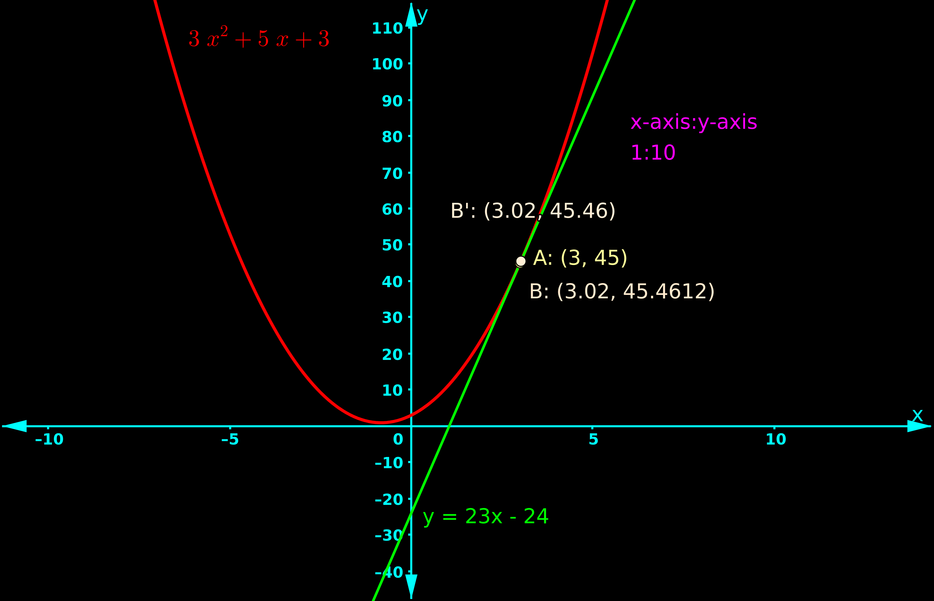
10. Fig.22.23 below shows the graph.
   ♦ f is drawn in red color
   ♦ L is drawn in green color

Fig.22.23

   ♦ A is a point on f
   ♦ B is a point on f
   ♦ B' is a point on L
• We want the y-coordinate at B. But, for ease of calculation, we use linear approximation and obtain the y-coordinate at B'.
• In the graph, A, B and B' are so close to each other that, they are not distinctly visible from each other.

 

Solved example 22.26
Write the linear approximation of f(x) = sin x and use it to estimate sin 62^o.
Solution:
1. Given $\rm{f(x) = \sin x}$
• We are asked to write the linear approximation of this function at an arbitrary point. Let us choose the arbitrary point x = a.
2. The slope at any point is $\rm{f'(x) ~=~\cos x}$  
• So the slope at 'a' is $\rm{f'(a) ~=~\cos a}$
3. At the point where x = a, the y coordinate can be calculated as follows:
y = sin x = sin a
4.  So the tangent at x = a can be obtained as:
$\begin{array}{ll} {~\color{magenta}    1    }    &{{}}    &{y - \sin a}    & {~=~}    &{\cos a \,(x - a)}    \\ {~\color{magenta}    2    }    &{\implies}    &{y}    & {~=~}    &{\cos a \, (x - a) + \sin a}    \\ {~\color{magenta}    3    }    &{{}}    &{{}}    & {~=~}    &{x \cos a ~-~ a \cos a ~+~\sin a}    \\ \end{array}$
5. So the linear approximation of f at x = a is:
$L(x) = x \cos a ~-~ a \cos a ~+~\sin a$
6. Using linear approximation, we can calculate f(b) because:
f(b) ≈ L(b) if b is close to a.
• In our present case, b = 62^o.
• Converting this to radians, we get:
$\rm{62^o ~=~62 \times \frac{\pi}{180}~=~\frac{62 \pi}{180}}$
• 'a' should be selected in such a way that:
   ♦ 'a' is a convenient number
   ♦ 'a' is close to 'b'.
• We can take a = 60^o
cosine and sine of 60 is already known. So it is a convenient number. Also, 60 is close to 62.
• Converting 60^o to radians, we have:
$\rm{60^o ~=~\frac{\pi}{3}}$
7. Based on the result in (5), we can write:
Linear approximation of f at x = π/3 is:
$\begin{array}{ll} {~\color{magenta}    1    }    &{{}}    &{L(x)}    & {~=~}    &{x \cos a ~-~ a \cos a ~+~\sin a}    \\ {~\color{magenta}    2    }    &{\implies}    &{L(x)_{a=\pi / 3}}    & {~=~}    &{x \cos \frac{\pi}{3} ~-~ a \cos \frac{\pi}{3} ~+~\sin \frac{\pi}{3}}    \\ {~\color{magenta}    3    }    &{{}}    &{{}}    & {~=~}    &{\frac{x}{2} ~-~ \frac{\pi}{6} ~+~ \frac{\sqrt3}{2}}    \\ \end{array}$
8. Based on what we wrote in (6), we get:
$\begin{array}{ll} {~\color{magenta}    1    }    &{{}}    &{f(b)}    & {~≈~}    &{L(b)}    \\ {~\color{magenta}    2    }    &{\implies}    &{f(\frac{62 \pi}{180})}    & {~≈~}    &{L(\frac{62 \pi}{180})}    \\ {~\color{magenta}    3    }    &{\implies}    &{\sin \frac{62 \pi}{180}}    & {~≈~}    &{\frac{62 \pi}{180} ~-~ \frac{\pi}{6} ~+~ \frac{\sqrt3}{2}}    \\ {~\color{magenta}    4    }    &{{}}    &{{}}    & {~≈~}    &{0.883478 }    \\ \end{array}$
9. It is interesting to note that, if we use a calculator or computer to calculate the sine of 62^o, we will get:
$\sin 62^o~=~0.882947$

Solved example 22.27
Write the linear approximation of f(x) = cos x and use it to estimate cos 89^o.
Solution:
1. Given $\rm{f(x) = \cos x}$
• We are asked to write the linear approximation of this function at an arbitrary point. Let us choose the arbitrary point x = a.
2. The slope at any point is $\rm{f'(x) ~=~-\sin x}$  
• So the slope at 'a' is $\rm{f'(a) ~=~-\sin a}$
3. At the point where x = a, the y coordinate can be calculated as follows:
y = cos x = cos a
4.  So the tangent at x = a can be obtained as:
$\begin{array}{ll} {~\color{magenta}    1    }    &{{}}    &{y - \cos a}    & {~=~}    &{-\sin a \,(x - a)}    \\ {~\color{magenta}    2    }    &{\implies}    &{y}    & {~=~}    &{-\sin a \, (x - a) + \cos a}    \\ {~\color{magenta}    3    }    &{{}}    &{{}}    & {~=~}    &{-x \sin a ~+~ a \sin a ~+~\cos a}    \\ \end{array}$
5. So the linear approximation of f at x = a is:
$L(x) = -x \sin a ~+~ a \sin a ~+~\cos a$
6. Using linear approximation, we can calculate f(b) because:
f(b) ≈ L(b) if b is close to a.
• In our present case, b = 89^o.
• Converting this to radians, we get:
$\rm{89^o ~=~89 \times \frac{\pi}{180}~=~\frac{89 \pi}{180}}$
• 'a' should be selected in such a way that:
   ♦ 'a' is a convenient number
   ♦ 'a' is close to 'b'.
• We can take a = 90^o
cosine and sine of 90 is already known. So it is a convenient number. Also, 90 is close to 89.
• Converting 90^o to radians, we have:
$\rm{90^o ~=~\frac{\pi}{2}}$
7. Based on the result in (5), we can write:
Linear approximation of f at x = π/2 is:
$\begin{array}{ll} {~\color{magenta}    1    }    &{{}}    &{L(x)}    & {~=~}    &{-x \sin a ~+~ a \sin a ~+~\cos a}    \\ {~\color{magenta}    2    }    &{\implies}    &{L(x)_{a=\pi / 2}}    & {~=~}    &{-x \sin \frac{\pi}{2} ~+~ a \sin \frac{\pi}{2} ~+~\cos \frac{\pi}{2}}    \\ {~\color{magenta}    3    }    &{{}}    &{{}}    & {~=~}    &{-x ~+~ \frac{\pi}{2}}    \\ \end{array}$
8. Based on what we wrote in (6), we get:
$\begin{array}{ll} {~\color{magenta}    1    }    &{{}}    &{f(b)}    & {~≈~}    &{L(b)}    \\ {~\color{magenta}    2    }    &{\implies}    &{f(\frac{89 \pi}{180})}    & {~≈~}    &{L(\frac{89 \pi}{180})}    \\ {~\color{magenta}    3    }    &{\implies}    &{\cos \frac{89 \pi}{180}}    & {~≈~}    &{-\frac{89 \pi}{180} ~+~ \frac{\pi}{2}}    \\ {~\color{magenta}    4    }    &{{}}    &{{}}    & {~≈~}    &{0.01745329}    \\ \end{array}$
9. It is interesting to note that, if we use a calculator or computer to calculate the cosine of 89^o, we will get:
$\cos 89^o~=~0.017452406$

Solved example 22.28
Write the linear approximation of f(x) = (1+x)ⁿ and use it to estimate (1.01)³.
Solution:
1. Given $\rm{f(x) = (1+x)^n}$
• We are asked to write the linear approximation of this function at an arbitrary point. Let us choose the arbitrary point x = a.
2. The slope at any point is $\rm{f'(x) ~=~n(1+x)^{n-1}}$  
• So the slope at 'a' is $\rm{f'(a) ~=~n(1+a)^{n-1}}$
3. At the point where x = a, the y coordinate can be calculated as follows:
$\rm{y = (1+a)^n}$
4.  So the tangent at x = a can be obtained as:
$\begin{array}{ll} {~\color{magenta}    1    }    &{{}}    &{y - (1+a)^n}    & {~=~}    &{n(1+a)^{n-1} \,(x - a)}    \\ {~\color{magenta}    2    }    &{\implies}    &{y}    & {~=~}    &{nx(1+a)^{n-1}~-~na(1+a)^{n-1}~+~(1+a)^{n}}    \\ \end{array}$
5. So the linear approximation of f at x = a is:
$L(x) = nx(1+a)^{n-1}~-~na(1+a)^{n-1}~+~(1+a)^{n}$
6. Using linear approximation, we can calculate f(b) because:
f(b) ≈ L(b) if b is close to a.
• In our present case, b = 0.01.
• 'a' should be selected in such a way that:
   ♦ 'a' is a convenient number
   ♦ 'a' is close to 'b'.
• We can take a = 0
Then (1+a) will become 1. So it is a convenient number. Also, 0 is close to 0.01.
7. Based on the result in (5), we can write:
Linear approximation of f at x = 0 is:
$\begin{array}{ll} {~\color{magenta}    1    }    &{{}}    &{L(x)}    & {~=~}    &{nx(1+a)^{n-1}~-~na(1+a)^{n-1}~+~(1+a)^{n}}    \\ {~\color{magenta}    2    }    &{\implies}    &{L(x)_{a=0}}    & {~=~}    &{nx(1) ~-~n(0)(1)~+~1}    \\ {~\color{magenta}    3    }    &{{}}    &{{}}    & {~=~}    &{nx ~+~ 1}    \\ \end{array}$
8. Based on what we wrote in (6), we get:
$\begin{array}{ll} {~\color{magenta}    1    }    &{{}}    &{f(b)}    & {~≈~}    &{L(b)}    \\ {~\color{magenta}    2    }    &{\implies}    &{f(0.01)}    & {~≈~}    &{L(0.01)}    \\ {~\color{magenta}    3    }    &{\implies}    &{(1+0.01)^n}    & {~≈~}    &{n(0.01) + 1}    \\ {~\color{magenta}    4    }    &{{\implies}}    &{{(1.01)^3}}    & {~≈~}    &{3(0.01) + 1}    \\ {~\color{magenta}    5    }    &{{}}    &{{}}    & {~≈~}    &{1.03}    \\ \end{array}$
9. It is interesting to note that, if we use a calculator or computer to calculate (1.01)³, we will get:
$(1.01)^3~=~1.030301$

Solved example 22.29
Write the linear approximation of f(x) = (1−x)^1/10 and use it to estimate (0.999)^1/10.
Solution:
1. Given $\rm{f(x) = (1-x)^{1/10}}$
• We are asked to write the linear approximation of this function at an arbitrary point. Let us choose the arbitrary point x = a.
2. The slope at any point is:
$\rm{f'(x) ~=~\frac{1}{10}(1- x)^{-9/10} (-1)~=~\frac{-1}{10}(1- x)^{-9/10}}$  
• So the slope at 'a' is $\rm{f'(a) ~=~\frac{-1}{10}(1- a)^{-9/10}}$
3. At the point where x = a, the y coordinate can be calculated as follows:
$\rm{y = (1-a)^{1/10}}$
4.  So the tangent at x = a can be obtained as:
$\begin{array}{ll} {~\color{magenta}    1    }    &{{}}    &{y - (1-a)^{1/10}}    & {~=~}    &{\frac{-1}{10}(1- a)^{-9/10} \,(x - a)}    \\ {~\color{magenta}    2    }    &{\implies}    &{y}    & {~=~}    &{\frac{-1}{10}(1- a)^{-9/10} \,(x - a)~+~(1-a)^{1/10}}    \\ \end{array}$
5. So the linear approximation of f at x = a is:
$L(x) = \frac{-1}{10}(1- a)^{-9/10} \,(x - a)~+~(1-a)^{1/10}$
6. Using linear approximation, we can calculate f(b) because:
f(b) ≈ L(b) if b is close to a.
• In our present case, b = 0.001.
This is because, 0.999 = (1 − 0.001)
• 'a' should be selected in such a way that:
   ♦ 'a' is a convenient number
   ♦ 'a' is close to 'b'.
• We can take a = 0
Then (1−a) will become 1. So it is a convenient number. Also, 0 is close to 0.001.
7. Based on the result in (5), we can write:
Linear approximation of f at x = 0 is:
$\begin{array}{ll} {~\color{magenta}    1    }    &{{}}    &{L(x)}    & {~=~}    &{\frac{-1}{10}(1- a)^{-9/10} \,(x - a)~+~(1-a)^{1/10}}    \\ {~\color{magenta}    2    }    &{\implies}    &{L(x)_{a=0}}    & {~=~}    &{\frac{-1}{10}(1) \,(x)~+~1}    \\ {~\color{magenta}    3    }    &{{}}    &{{}}    & {~=~}    &{\frac{-x}{10} ~+~ 1}    \\ \end{array}$
8. Based on what we wrote in (6), we get:
$\begin{array}{ll} {~\color{magenta}    1    }    &{{}}    &{f(b)}    & {~≈~}    &{L(b)}    \\ {~\color{magenta}    2    }    &{\implies}    &{f(0.001)}    & {~≈~}    &{L(0.001)}    \\ {~\color{magenta}    3    }    &{\implies}    &{(1-0.001)^{1/10}}    & {~≈~}    &{\frac{-0.001}{10} + 1}    \\ {~\color{magenta}    4    }    &{{\implies}}    &{{(0.999)^{1/10}}}    & {~≈~}    &{-0.0001 + 1}    \\ {~\color{magenta}    5    }    &{{}}    &{{}}    & {~≈~}    &{0.9999}    \\ \end{array}$
9. It is interesting to note that, if we use a calculator or computer to calculate (0.999)^1/10, we will get:
$(0.999)^{1/10}~=~0.9998999$
10. Fig.22.24 below shows the graph.
   ♦ f is drawn in red color
   ♦ L is drawn in green color

Fig.22.24

   ♦ A is a point on f
   ♦ B is a point on f
   ♦ B' is a point on L
• We want the y-coordinate at B. But, for ease of calculation, we use linear approximation and obtain the y-coordinate at B'.
• In the graph, A, B and B' are so close to each other that, they are not distinctly visible from each other.

---

In the next section, we will see Differentials.

Previous

Contents

Next

Copyright©2024 Higher secondary mathematics.blogspot.com