Showing posts with label polynomial. Show all posts

Thursday, November 18, 2021

Chapter 2.4 - Rational Function

In the previous section, we saw constant function and polynomial function. In this section, we will see rational function.

D. Rational function
• A rational function is a real valued function f: R→R defined by:
$\mathbf\small{\rm{f(x)=\frac{p(x)}{q(x)}}}$
• Details can be written in 11 steps:
1. Given that, it is a real valued function. That means, all values obtained after processing, must be real values.
2. Let us examine the numerator and denominator:
• The numerator is p(x). It must be a polynomial function.
• The denominator is q(x). It must also be a polynomial function.
   ♦ This q(x) should not be equal to zero.
   ♦ If it is zero, the function f(x) cannot be defined.
3. The function can be defined by writing the ordered pairs which satisfy that function.
• So our next task is to find those ordered pairs.
• We will take a simple rational function: f(x) = $\mathbf\small{\rm{\frac{1}{x}}}$
    ♦ Recall that all constants are polynomials. So '1' is a polynomial.
    ♦ For example, 4 can be written as: 4x0, which is (4 × 1) = 4
4. It is given that, f : R→R
• This indicates that,
   ♦ the first elements of the ordered pairs (input x values) should be taken from the set R.
   ♦ the second elements (resulting y values) should be present in the set R
5. The set R is the set of real numbers. It will include integers, negative values, positive values, fractions, decimals, recurring decimals, numbers like √2, √5, π etc.,. In short, R will contain every value which can be plotted on a number line. Recall that we plotted √2, √5, π etc., in our previous classes.
• Since different types of numbers are present in R, we will choose some convenient numbers at random.
• Let x = -7
   ♦ This x is processed as follows:
   ♦ f(-7) = $\mathbf\small{\rm{\frac{1}{(-7)}}}$ = -0.143
   ♦ f(-7) is the 'y value' when 'x value' is -7
   ♦ So we get an ordered pair (x,y) as: (-7, -0.143)
• Let x = -5
   ♦ This x is processed as follows:
   ♦ f(-5) = $\mathbf\small{\rm{\frac{1}{(-5)}}}$ = -0.2
   ♦ f(-5) is the 'y value' when 'x value' is -5
   ♦ So we get an ordered pair (x,y) as: (-5, -0.2)
• Let x = 1
   ♦ This x is processed as follows:
   ♦ f(1) = $\mathbf\small{\rm{\frac{1}{(1)}}}$ = 1
   ♦ f(1) is the 'y value' when 'x value' is 1
   ♦ So we get an ordered pair (x,y) as: (1, 1)
• Let x = 2
   ♦ This x is processed as follows:
   ♦ f(2) = $\mathbf\small{\rm{\frac{1}{(2)}}}$ = 0.5
   ♦ f(2) is the 'y value' when 'x value' is 2
   ♦ So we get an ordered pair (x,y) as: (2, 0.5)
• Let x = 5
   ♦ This x is processed as follows:
   ♦ f(5) = $\mathbf\small{\rm{\frac{1}{(5)}}}$ = 0.2
   ♦ f(5) is the 'y value' when 'x value' is 0.2
   ♦ So we get an ordered pair (x,y) as: (5, 0.2)
• Let x = 10
   ♦ This x is processed as follows:
   ♦ f(10) = $\mathbf\small{\rm{\frac{1}{(10)}}}$ = 0.1
   ♦ f(10) is the 'y value' when 'x value' is 10
   ♦ So we get an ordered pair (x,y) as: (10, 0.1)
• We see that, whatever be the value of x, the value of y will be the reciprocal of that x value.
6. Proceeding like this, we will get infinite number of ordered pairs. All those ordered pairs should be included in the set f.
• So we can write: f = {. . . , (-7,-0.143), (-5, -0.2), (1, 1), (2, 0.5), (5, 0.2), (10, 0.1), . . .}
7. The above set f is written in roster form. But we have to remember an important point. It can be written in 3 steps:
(i) Both elements of the ordered pairs are real numbers.
(ii) Since they are real numbers, there will be integers, negative values, positive values, fractions, decimals, recurring decimals, numbers like √2, √5, π etc.,. We cannot think of a definite sequence to write them.
(iii) So it is better to use set builder form to write f.
8. In the set builder form, we can write:
f = {(x,y) : x ∈ R, y = $\mathbf\small{\rm{\frac{1}{x}}}$, $\mathbf\small{\rm{\frac{1}{x}}}$ ∈ R}
• That means:
    ♦ The set f contains all ordered pairs (x,y) such that,
    ♦ x is a real number,
    ♦ y is the reciprocal of x,
    ♦ reciprocal of x is a real number
• But there is a problem. We cannot put x = 0. The function is not defined at x = 0.
• This problem can be solved in 3 steps:
(i) Consider the set R - {0}.
    ♦ Here we are subtracting the 'set containing zero' from the set R
(ii) The resulting set will not contain zero.
    ♦ We must take x only from R - {0}
(iii) So we must modify the above set builder form. We get:
f = {(x,y) : x ∈ R - {0}, y = $\mathbf\small{\rm{\frac{1}{x}}}$, $\mathbf\small{\rm{\frac{1}{x}}}$ ∈ R}
• That means:
    ♦ The set f contains all ordered pairs (x,y) such that,
    ♦ x is an element of R - {0},
    ♦ y is the reciprocal of x,
    ♦ reciprocal of x is a real number
9. Once we write the set f, we can write the domain and range of f.
(i) First we will write the domain:
• Domain of f is the set containing all the first elements of the ordered pairs in f.
• In our present case, there are infinite number of ordered pairs. So there will be infinite number of first elements.
• We saw that all the first elements are real numbers (except zero). Since they are real numbers, there will be integers, negative values, positive values, fractions, decimals, recurring decimals, numbers like √2, √5, π etc.,. We cannot think of a definite sequence to write them. So it is better to use set builder form rather than the roster form.
• We can write:
    ♦ Domain of f = {x : x ∈ R - {0}}
• That means:
    ♦ The domain of f will contain all real numbers except zero.
(ii) Next we will write the range:
• Range of f is the set containing all the second elements of the ordered pairs in f.
• In our present case, there are infinite number of ordered pairs. So there will be infinite number of second elements.
• We saw that all the first elements are real numbers (except zero). Since the second elements are reciprocals, they will also be real numbers. So there will be integers, negative values, positive values, fractions, decimals, recurring decimals etc.,. We cannot think of a definite sequence to write them. So it is better to use set builder form rather than the roster form.
• We can write:
    ♦ Range of f = {$\mathbf\small{\rm{\frac{1}{x}}}$ : x ∈ R - {0}}
• That means:
    ♦ The range of f will contain reciprocals of all real numbers except zero.
10. We can make a table using the x and y values in the set f. Such a table is convenient to draw the graph of the function.
• Note that, to input for x, we choose convenient numbers from the set R - {0}.
• It is better not to choose numbers with recurring decimals. They will be difficult to plot.

Table 2.6

11. The red curves in fig.2.14(a) below, is the graph of the function.

Fig.2.14

• The graph in fig.b is drawn to a different scale. This can be explained in 5 steps:
(i) The y value is the reciprocal of x value. So we will need many small values on the y axis.
(ii) To achieve this within limited space, we change the scale of the y axis.
(iii) In the fig.2.14(a), we have:
    ♦ Scale of x axis as: 1 cm = 1 unit
    ♦ Scale of y axis as: 1 cm = 1 unit
(iv) In the fig.2.13(b), we have:
    ♦ Scale of x axis as: 1 cm = 1 unit
    ♦ Scale of y axis as: 1 cm = 0.25 unit
(v) So the graph in fig.b is a bit distorted. But the coordinates do not change.
• The reader is advised to prepare a table and draw the graph in his/her own graph books.
• We can write some peculiarities of this red curve. They can be written in 3 steps:
(i) The red curve of f(x) = $\mathbf\small{\rm{\frac{1}{x}}}$ never passes through the origin (0,0)
(ii) Mark any point on the red curve. Note the coordinates of that point.
   ♦ The y coordinate will be the reciprocal of the x coordinate.
   ♦ This is shown in fig.b
   ♦ The green vertical dashed line shows 2
         ✰ The green horizontal dashed line shows the reciprocal 0.5
   ♦ The magenta vertical dashed line shows -5
         ✰ The magenta horizontal dashed line shows the reciprocal -0.2
(iii) We see arrows at both ends of the red curves. There are four arrows. We will call them I, II, III and IV.
I. The top arrow of the right side red curve:
• This arrow indicates that, the curve can go very high up.
• This can be explained as follows:
   ♦ As we move along this curve from right towards the left, x takes values closer and closer to zero.
         ✰ For example, 0.00001 is closer to zero than 0.0001
   ♦ Values closer to zero are very small.
         ✰ The reciprocals of such small values will be very large.
   ♦ The reciprocals are y values.
         ✰ That means y values will be very large.
         ✰ They are very high up in the graph.
         ✰ This arrow indeed indicates that the graph will go very high up (y = +∞).
   ♦ As the x takes values closer and closer to zero, we get the feeling that, this end of the curve is going to touch the y axis.
         ✰ It will touch the y axis when x = 0
         ✰ However, x cannot become equal to zero.
         ✰ If it is zero, then the function can not be defined.
         ✰ This is because, $\mathbf\small{\rm{\frac{1}{x}}}$ becomes $\mathbf\small{\rm{\frac{1}{0}}}$
   ♦ So this end will never touch the y axis
         ✰ When we draw this graph on a sheet of paper or the computer screen, it appears to touch.
         ✰ But if we zoom in, we will see that, there is a little gap.
II
. The bottom arrow of the right side red curve:
• This arrow indicates that, the curve can reach to the point where (x = +∞).
• This can be explained as follows:
   ♦ As we move along this curve from left towards the right, x take values closer and closer to +∞.
   ♦ Values closer to +∞ are very large.
         ✰ The reciprocals of such small values will be very small.
   ♦ The reciprocals are y values.
         ✰ That means y values will be very small.
         ✰ They get closer and closer to zero.
   ♦ As the y becomes closer and closer to zero, we get the feeling that, this end of the curve is going to touch the x axis.
         ✰ It will touch the x axis when x = +∞
         ✰ However, x cannot become equal to +∞.
   ♦ So this end will never touch the x axis
         ✰ When we draw this graph on a sheet of paper or the computer screen, it appears to touch.
         ✰ But if we zoom in, we will see that, there is a little gap.
III
. The top arrow of the left side red curve:
• This arrow indicates that, the curve can reach to the point where (x = -∞).
• This can be explained as follows:
   ♦ As we move along this curve from right towards the left, x take values closer and closer to -∞.
   ♦ Values closer to -∞ are very large (numerically).
         ✰ The reciprocals of such small values will be very small.
   ♦ The reciprocals are negative y values.
         ✰ That means negative y values will be very small.
         ✰ They get closer and closer to zero.
   ♦ As the y becomes closer and closer to zero, we get the feeling that, this end of the curve is going to touch the x axis.
         ✰ It will touch the x axis when x = -∞
         ✰ However, x cannot become equal to -∞.
   ♦ So this end will never touch the x axis
         ✰ When we draw this graph on a sheet of paper or the computer screen, it appears to touch.
         ✰ But if we zoom in, we will see that, there is a little gap.
IV
. The bottom arrow of the left side red curve:
• This arrow indicates that, the curve can go very low bottom.
• This can be explained as follows:
   ♦ As we move along this curve from left towards the right, x takes values closer and closer to zero.
         ✰ For example, -0.0001 is closer to zero than -0.00001
   ♦ Values closer to zero are very small.
         ✰ The reciprocals of such small values will be very large.
   ♦ The reciprocals are negative y values.
         ✰ That means negative y values will be very large (numerically).
         ✰ They are very low down in the graph.
         ✰ This arrow indeed indicates that the graph will go very low bottom (y = -∞).
   ♦ As the x takes values closer and closer to zero, we get the feeling that, this end of the curve is going to touch the y axis.
         ✰ It will touch the y axis when x = 0
         ✰ However, x cannot become equal to zero.
         ✰ If it is zero, then the function can not be defined.
         ✰ This is because, $\mathbf\small{\rm{\frac{1}{x}}}$ becomes $\mathbf\small{\rm{\frac{1}{0}}}$
   ♦ So this end will never touch the y axis
         ✰ When we draw this graph on a sheet of paper or the computer screen, it appears to touch.
         ✰ But if we zoom in, we will see that, there is a little gap.
10. The rational function f(x) = $\mathbf\small{\rm{\frac{1}{x}}}$ has many applications in science and engineering.


In the next section, we will see a few more common functions.

Previous

Contents

Next

Copyright©2021 Higher secondary mathematics.blogspot.com

Wednesday, November 17, 2021

Chapter 2.3 - Polynomial Function

In the previous section, we saw the basics about functions. We also saw the features of identity function. In this section, we will see constant function and polynomial function.

B. Constant function
This is a real valued function f: R→R defined by y = f (x) = c
Details can be written in 11 steps:
1. Given that, it is a real valued function. That means, all values obtained after processing, must be real values.
• The function can be defined by writing the ordered pairs which satisfy that function.
• So our next task is to find those ordered pairs.
2. It is given that, f : R→R
• This indicates that,
   ♦ the first elements of the ordered pairs (input x values) should be taken from the set R.
   ♦ the second elements (resulting y values) should be present in the set R
3. The set R is the set of real numbers. It will include integers, negative values, positive values, fractions, decimals, recurring decimals, numbers like √2, √5, π etc.,. In short, R will contain every value which can be plotted on a number line. Recall that we plotted √2, √5, π etc., in our previous classes.
• Since different types of numbers are present in R, we will choose some convenient numbers at random.
• Let x = -7
   ♦ This x is processed as follows:
   ♦ f(-7) = c
   ♦ f(-7) is the 'y value' when 'x value' is -7
   ♦ So we get an ordered pair (x,y) as: (-7,c)
• Let x = -3
   ♦ This x is processed as follows:
   ♦ f(-3) = c
   ♦ f(-3) is the 'y value' when 'x value' is -3
   ♦ So we get another ordered pair (x,y) as: (-3,c)
• Let x = 1.414
   ♦ This x is processed as follows:
   ♦ f(1.414) = c
   ♦ f(1.414) is the 'y value' when 'x value' is 1.414
   ♦ So we get another ordered pair (x,y) as: (1.414,c)
• We see that, whatever be the value of x, the value of y will always be c.
4. Proceeding like this, we will get infinite number of ordered pairs. All those ordered pairs should be included in the set f.
• So we can write: f = {. . . , (-7,c), (-3,c), (1.414,c), (5,c), . . .}
5. In step (2), we noted that, the second elements of the ordered pairs must also be from set R.
• Here we have only one second element, which is 'c'.
   ♦ But this 'c' must be from R.
   ♦ That means, 'c' must be a real number.
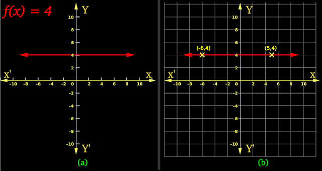
• Let us put c = 4. Then the function becomes f(x) = 4
• We can write: f = {. . . , (-7,4), (-3,4), (1.414,4), (5,4), . . .}
6. The above set f is written in roster form. But we have to remember an important point. It can be written in 3 steps:
(i) Both elements of the ordered pairs are real numbers.
(ii) Since they are real numbers, there will be integers, negative values, positive values, fractions, decimals, recurring decimals, numbers like √2, √5, π etc.,. We cannot think of a definite sequence to write them.
(iii) So it is better to use set builder form to write f.
7. In the set builder form, we can write:
f = {(x,y) : x ∈ R, y = c, c ∈ R}
• That means:
    ♦ The set f contains all ordered pairs (x,y) such that,
    ♦ x is a real number,
    ♦ y is a constant c,
    ♦ c is a real number
8. Once we write the set f, we can write the domain and range of f.
(i) First we will write the domain:
• Domain of f is the set containing all the first elements of the ordered pairs in f.
• In our present case, there are infinite number of ordered pairs. So there will be infinite number of first elements.
• We saw that all the first elements are real numbers. Since they are real numbers, there will be integers, negative values, positive values, fractions, decimals, recurring decimals, numbers like √2, √5, π etc.,. We cannot think of a definite sequence to write them. So it is better to use set builder form rather than the roster form.
• We can write:
    ♦ Domain of f = {x : x ∈ R}
• That means:
    ♦ The domain of f is the set of all x such that,
    ♦ x is a real number.
(ii) Next we will write the range:
• Range of f is the set containing all the second elements of the ordered pairs in f.
• In our present case, there are infinite number of c. But in a set, we write repeating elements only once.
• We can write:
    ♦ Range of f = {c}
9. We can make a table using the x and y values in the set f. Such a table is convenient to draw the graph of the function.
• Note that, to input for x, we choose convenient numbers from the set R.
• It is better not to choose numbers with recurring decimals. They will be difficult to plot.

Table 2.3
 10. The red line in fig.2.11(a) below, is the graph of this function.

Graph of constant function is a horizontal line.
Fig.2.11
• The reader is advised to prepare a table and draw the graph in his/her own graph books.
• We can write some peculiarities of this red line. They can be written in 6 steps:
(i) The red line will be always horizontal and passes through y = c
(ii) Mark different points on the red line. Note the coordinates of those points.
   ♦ All y coordinates will be the same c.
   ♦ This is shown in fig.b
(iii) We see arrows at both ends of the red line.
• The arrow at the left end of the red line indicates that, the line can extend up to the point where x = -∞ and y = c.
• The arrow at the right end of the red line indicates that, the line can extend up to the point where x = +∞ and y = c.
11. The constant function has many applications in science and engineering.

C. Polynomial function
• We have seen some basics about polynomials in our earlier classes (Details here).
• A polynomial function is a real valued function f: R→R defined by:
y = f (x) = a0 + a1x + a2x2 + a3x3 + . . . + anxn
• Details can be written in 11 steps:
1. Given that, it is a real valued function. That means, all values obtained after processing, must be real values.
• The function can be defined by writing the ordered pairs which satisfy that function.
• So our next task is to find those ordered pairs.
• We will take a simple polynomial function: f(x) = x2
2. It is given that, f : R→R
• This indicates that,
   ♦ the first elements of the ordered pairs (input x values) should be taken from the set R.
   ♦ the second elements (resulting y values) should be present in the set R
3. The set R is the set of real numbers. It will include integers, negative values, positive values, fractions, decimals, recurring decimals, numbers like √2, √5, π etc.,. In short, R will contain every value which can be plotted on a number line. Recall that we plotted √2, √5, π etc., in our previous classes.
• Since different types of numbers are present in R, we will choose some convenient numbers at random.
• Let x = -7
   ♦ This x is processed as follows:
   ♦ f(-7) = (-7)2 = 49
   ♦ f(-7) is the 'y value' when 'x value' is -7
   ♦ So we get an ordered pair (x,y) as: (-7,49)
• Let x = -3
   ♦ This x is processed as follows:
   ♦ f(-3) = (-3)2 = 9
   ♦ f(-3) is the 'y value' when 'x value' is -3
   ♦ So we get an ordered pair (x,y) as: (-3,9)
• Let x = 1.414
   ♦ This x is processed as follows:
   ♦ f(1.414) = (1.414)2 = 2
   ♦ f(1.414) is the 'y value' when 'x value' is 1.414
   ♦ So we get an ordered pair (x,y) as: (1.414,2)
• We see that, whatever be the value of x, the value of y will be the square of that x value.
4. Proceeding like this, we will get infinite number of ordered pairs. All those ordered pairs should be included in the set f.
• So we can write: f = {. . . , (-7,49), (-3,9), (1.414,2), (5,25), . . .}
5. The above set f is written in roster form. But we have to remember an important point. It can be written in 3 steps:
(i) Both elements of the ordered pairs are real numbers.
(ii) Since they are real numbers, there will be integers, negative values, positive values, fractions, decimals, recurring decimals, numbers like √2, √5, π etc.,. We cannot think of a definite sequence to write them.
(iii) So it is better to use set builder form to write f.
6. In the set builder form, we can write:
f = {(x,y) : x ∈ R, y = x2, x2 ∈ R}
• That means:
    ♦ The set f contains all ordered pairs (x,y) such that,
    ♦ x is a real number,
    ♦ y is the square of x,
    ♦ square of x is a real number
7. Once we write the set f, we can write the domain and range of f.
(i) First we will write the domain:
• Domain of f is the set containing all the first elements of the ordered pairs in f.
• In our present case, there are infinite number of ordered pairs. So there will be infinite number of first elements.
• We saw that all the first elements are real numbers. Since they are real numbers, there will be integers, negative values, positive values, fractions, decimals, recurring decimals, numbers like √2, √5, π etc.,. We cannot think of a definite sequence to write them. So it is better to use set builder form rather than the roster form.
• We can write:
    ♦ Domain of f = {x : x ∈ R}
• That means:
    ♦ The domain of f will contain all real numbers.
(ii) Next we will write the range:
• Range of f is the set containing all the second elements of the ordered pairs in f.
• In our present case, there are infinite number of ordered pairs. So there will be infinite number of second elements.
• We saw that all the first elements are real numbers. Since the second elements are squares, there will not be any negative numbers. But there will be integers,  fractions, decimals, recurring decimals etc.,. We cannot think of a definite sequence to write them. So it is better to use set builder form rather than the roster form.
• We can write:
    ♦ Range of f = {x2 : x ∈ R}
• That means:
    ♦ The domain of f will contain squares of all real numbers.
8. We can make a table using the x and y values in the set f. Such a table is convenient to draw the graph of the function.
• Note that, to input for x, we choose convenient numbers from the set R.
• It is better not to choose numbers with recurring decimals. They will be difficult to plot.

Table 2.4
 9. The red curve in fig.2.12(a) below, is the graph of the function.

Fig.2.12

• The reader is advised to prepare a table and draw the graph in his/her own graph books.
• We can write some peculiarities of this red curve. They can be written in 3 steps:
(i) The red curve of f(x) = x2 always passes through the origin (0,0)
(ii) Mark any point on the red curve. Note the coordinates of that point.
   ♦ The y coordinate will be the square of the x coordinate.
   ♦ This is shown in fig.b
   ♦ The green vertical dashed line shows 1.414
         ✰ The green horizontal dashed line shows the square 2
   ♦ The magenta vertical dashed line shows -4
         ✰ The magenta horizontal dashed line shows the square 16
(iii) We see arrows at both ends of the red curve.
• The arrow at the left end of the red curve indicates that, the curve can extend up to the point where x = -∞ and y = square of that x value.
• The arrow at the right end of the red curve indicates that, the curve can extend up to the point where x = +∞ and y = square of that x value.
10. The polynomial function f(x) = x2 has many applications in science and engineering.
11. We wrote the general form of polynomial functions as:
y = f (x) = a0 + a1x + a2x2 + a3x3 + . . . + anxn
◼ It is important to ensure that:
a0, a1, a2, a3, . . . , an are real numbers
    ♦ In other words, a0, a1, a2, a3, . . . , an ∈ R
◼ It is important to ensure that:
No exponent of x is negative.
◼ It is important to ensure that:
All exponents of x are integers.
[Recall the conditions for a polynomial that we saw in our previous classes. (Details here)]
• Some examples of polynomial functions are:
    ♦ f(x) = x3 – x2 + 2
    ♦ g(x) = x4 + √2 x
• The following function is not a polynomial function:
    ♦ $\mathbf\small{\rm{h(x)=x^{\frac{2}{3} }+2x}}$
    ♦ This is because, the exponent of x in the first term is not an integer


Let us see a solved example:
Solved example 2.28
Draw the graph of the real valued function f :R → R defined by f(x) = x3, x ∈ R.
Solution:
1. Given that, it is a real valued function. That means, all values obtained after processing, must be real values.
• The function can be defined by writing the ordered pairs which satisfy that function.
• So our next task is to find those ordered pairs.
• The given function is: f(x) = x3
2. It is given that, f: R→R
• This indicates that,
   ♦ the first elements of the ordered pairs (input x values) should be taken from the set R.
   ♦ the second elements (resulting y values) should be present in the set R
3. The set R is the set of real numbers. It will include integers, negative values, positive values, fractions, decimals, recurring decimals, numbers like √2, √5, π etc.,. In short, R will contain every value which can be plotted on a number line. Recall that we plotted √2, √5, π etc., in our previous classes.
• Since different types of numbers are present in R, we will choose some convenient numbers at random.
• Let x = -7
   ♦ This x is processed as follows:
   ♦ f(-7) = (-7)3 = -343
   ♦ f(-7) is the 'y value' when 'x value' is -7
   ♦ So we get an ordered pair (x,y) as: (-7, -343)
• Let x = -3
   ♦ This x is processed as follows:
   ♦ f(-3) = (-3)3 = -27
   ♦ f(-3) is the 'y value' when 'x value' is -3
   ♦ So we get an ordered pair (x,y) as: (-3, -27)
• Let x = 1.414
   ♦ This x is processed as follows:
   ♦ f(1.414) = (1.414)3 = 2.8271
   ♦ f(1.414) is the 'y value' when 'x value' is 1.414
   ♦ So we get an ordered pair (x,y) as: (1.414, 2.8271)
(Note that 1.414 is √2. So 2.8271 will be 2√2)
• We see that, whatever be the value of x, the value of y will be the cube of that x value.
4. Proceeding like this, we will get infinite number of ordered pairs. All those ordered pairs should be included in the set f.
• So we can write: f = {. . . , (-7, -343), (-3, -27), (1.414, 2.8271), (5, 125), . . .}
5. The above set f is written in roster form. But we have to remember an important point. It can be written in 3 steps:
(i) Both elements of the ordered pairs are real numbers.
(ii) Since they are real numbers, there will be integers, negative values, positive values, fractions, decimals, recurring decimals, numbers like √2, √5, π etc.,. We cannot think of a definite sequence to write them.
(iii) So it is better to use set builder form to write f.
6. In the set builder form, we can write:
f = {(x,y) : x ∈ R, y = x3, x3 ∈ R}
• That means:
    ♦ The set f contains all ordered pairs (x,y) such that,
    ♦ x is a real number,
    ♦ y is the cube of x,
    ♦ cube of x is a real number.
7. Once we write the set f, we can write the domain and range of f.
(i) First we will write the domain:
• Domain of f is the set containing all the first elements of the ordered pairs in f.
• In our present case, there are infinite number of ordered pairs. So there will be infinite number of first elements.
• We saw that all the first elements are real numbers. Since they are real numbers, there will be integers, negative values, positive values, fractions, decimals, recurring decimals, numbers like √2, √5, π etc.,. We cannot think of a definite sequence to write them. So it is better to use set builder form rather than the roster form.
• We can write:
    ♦ Domain of f = {x : x ∈ R}
• That means:
    ♦ The domain of f is the set of all x such that,
    ♦ x is a real number.
(ii) Next we will write the range:
• Range of f is the set containing all the second elements of the ordered pairs in f.
• In our present case, there are infinite number of ordered pairs. So there will be infinite number of second elements.
• We saw that all the first elements are real numbers. Since the second elements are cubes, there will be negative numbers also. There will be integers,  fractions, decimals, recurring decimals etc.,. We cannot think of a definite sequence to write them. So it is better to use set builder form rather than the roster form.
• We can write:
    ♦ Range of f = {x3 : x ∈ R}
• That means:
    ♦ The domain of f is the set of all x3 such that,
    ♦ x is a real number.
8. We can make a table using the x and y values in the set f. Such a table is convenient to draw the graph of the function.
• Note that, to input for x, we choose convenient numbers from the set R.
• It is better not to choose numbers with recurring decimals. They will be difficult to plot.

Table 2.5

9. The red curve in fig.2.13(a) below, is the graph of the function.

Fig.2.13

• The graph in fig.b is drawn to a different scale. This can be explained in 5 steps:
(i) The y value is cube of x value. So we will need more values on the y axis.
(ii) To achieve this within limited space, we change the scale of the y axis.
(iii) In the fig.2.13(a), we have:
    ♦ Scale of x axis as: 1 cm = 1 unit
    ♦ Scale of y axis as: 1 cm = 1 unit
(iv) In the fig.2.13(b), we have:
    ♦ Scale of x axis as: 1 cm = 1 unit
    ♦ Scale of y axis as: 1 cm = 10 unit
(v) So the graph in fig.b is a bit distorted. But the coordinates do not change.
• The reader is advised to prepare a table and draw the graph in his/her own graph books.
• We can write some peculiarities of this red curve. They can be written in 3 steps:
(i) The red curve of f(x) = x3 always passes through the origin (0,0)
(ii) Mark any point on the red curve. Note the coordinates of that point.
   ♦ The y coordinate will be the cube of the x coordinate.
   ♦ This is shown in fig.b
   ♦ The green vertical dashed line shows 3
         ✰ The green horizontal dashed line shows the cube 27
   ♦ The magenta vertical dashed line shows -4
         ✰ The magenta horizontal dashed line shows the cube -64
(iii) We see arrows at top and bottom of the red curve.
• The arrow at the top end of the red curve indicates that, the curve can extend up to the point where x = +∞ and y = cube of that x value.
• The arrow at the bottom end of the red curve indicates that, the curve can extend up to the point where x = -∞ and y = cube of that x value.
10. The polynomial function f(x) = x3 has many applications in science and engineering.


In the next section, we will see a Rational function.

Previous

Contents

Next

Copyright©2021 Higher secondary mathematics.blogspot.com